4 Context-dependent categorization
Categorization decisions are repelled away from the characteristics of temporal context. This pattern of results is consistent across the realm of perception, cognition and economics; yet the underlying computational mechanisms that produce it remain elusive. This chapter arbitrates between putative sources of contextual bias in categorization decisions based on the lightness, size or numerosity of visual stimuli, across two experiments. Our experimental design allowed us to rule out response bias as a driver of the effect. We considered two alternative explanations: contextual shifts in the category boundary (contraction bias) and contextual changes in our encoding and experience of the current stimulus (adaptation). We used changes in suprathreshold sensitivity to estimate the contribution of adaptation. Our results suggest that adaptive changes to the appearance of the to-be-categorized stimulus can account for up to half of the contextual bias in lightness categorization, and for ~10% and ~30% of the contextual bias in categorizations of stimulus size and numerosity.
4.1 Introduction
Sensory information is continuous, yet the choices we make based on it are necessarily discrete. In daily life, we seamlessly sort sensations into meaningful categories to guide our actions and behaviors. We do this by drawing boundaries through sensory space that divide the continuum of our experiences into distinct classifications. The location of those boundaries, however, is not static. It shifts over the course of our lifetime, starting with early cognitive development (Gopnik and Meltzoff 1987; Slawinski and Fitzgerald 1998), through our lived experiences (Pollak and Kistler 2002) and domain-specific expertise (Chi, Feltovich, and Glaser 1981; Shafto and Coley 2003). As we learn about the world, or a particular corner or field within it, our standards about what constitutes a particular category evolve, perhaps becoming more fine-tuned and consistent (Slawinski and Fitzgerald 1998; Shafto and Coley 2003).
Interestingly, category boundaries may also shift on a much finer time-scale, depending on our most recent experiences. In the domain of visual perception, for instance, the same square stimulus can be categorized as small or large depending on the size of the squares that precede it (Fig. 4.1a). If it happens to occur after several large squares, it would, on average, be more often categorized as small than if it happens to occur after several small squares. In the laboratory, this phenomenon has been examined by asking participants to categorize (or label) series of visual stimuli, presented one after the other. The experimenter would manipulate the distribution of stimulus characteristics: in some blocks, the participant may be presented with predominantly large stimuli; in others, they may be presented with predominantly small stimuli. The location of the category boundary in each experimental condition can then be quantified based on participant responses by estimating what stimulus size would lead to an equal proportion of “large” and “small” categorizations (known as the threshold or point of subjective equivalence/indifference point). The results of these experiments indicate the dynamic malleability of our categorization decisions. The location of the category boundary shifts predictably, tracking the central tendency of the distribution of stimulus characteristics present in the temporal context.
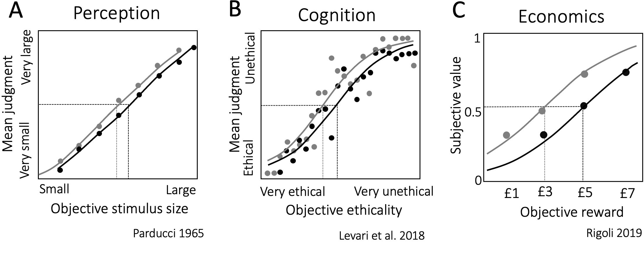
Figure 4.1: Context-dependent categorization across domains. Across all panels, the x-axis indexes the objective stimulus property and the y-axis – categorization decisions. \(\textbf{A:}\) Perception. Participants were asked to rate square stimuli on a scale between very large and very small. The psychometric curves depict participants’ categorization decisions across two contexts. The grey curve tracks judgments in a context dominated by objectively smaller stimuli, the black curve tracks judgments in a context dominated by objectively larger stimuli. Data from Parducci 1965, Fig. 7. \(\textbf{B:}\) Cognition. Participants were asked to accept or reject proposals for scientific studies that varied on a continuum of very ethical to very unethical (according to an independent group of raters). The shading of the curve again tracks context (grey: low prevalence of unethical studies, black: high prevalence of unethical studies). Data from Levari et al. 2018, Fig. 3b. \(\textbf{C:}\) Economics. The psychometric functions here depict participants’ subjective values estimated from choice behavior. Shading again tracks context (grey: low value context, black: high value context). Data from Rigoli 2019, Fig. 3a.
This pattern of results is robust. It generalizes across tasks that feature different types of visual stimuli (e.g. spatial frequency, Lages and Treisman 1998; distance, Morgan, Watamaniuk, and McKee 2000; hue, M. Olkkonen, McCarthy, and Allred 2014; facial expression, Levari et al. 2018) or engage other sensory modalities (e.g. weight perception, Helson 1947; interval timing, Jazayeri and Shadlen 2010). It holds regardless of whether participants are asked to use their “internal concept” of the category (Levari et al. 2018), whether they are provided with an explicit or implicit standard for categorization, or with feedback on the accuracy of their judgments (Morgan, Watamaniuk, and McKee 2000). It also extends beyond perception, when we need to abstract away from sensory information to evaluate, for instance, scenarios based on their ethicality (Fig. 4.1b, Levari et al. 2018) or economic prospects based on their subjective value (Fig. 4.1c, Rigoli 2019). Temporal context sways judgments across perception, cognition and economics in a predictable fashion. Category boundaries track the frequency and dispersion of recently experienced stimulus properties (Parducci 1965; Rigoli 2019), and so categorizations are repulsed away from recent experience. The smaller the squares we just saw, the more likely we would be to categorize a medium square as large. The more unethical the scenarios we just heard, the more likely we would be to judge an ambivalent scenario as ethical. The smaller the financial rewards we just experienced, the more likely we would be to perceive a moderate sum as valuable.
What drives this pattern of context dependence? One possibility is that it is driven by a response bias, whereby we calibrate our categorization judgments, such that the relative frequency of our actions remain stable across contexts. For instance, if we were faced with the choice of whether to accept or reject a proposal based on its ethicality, we might accept about half the proposals we encounter. But if the ethicality of proposals is particularly low in a given context (as it would be in the above described experimental manipulations) and we are compelled to accept half, this would naturally lead us to exhibit a lower threshold for (acceptable) ethicality. This is particularly likely in the laboratory, where response biases abound (Poulton and Poulton 1989; Bonnet 1990), as participants bring their priors (how likely is this category?), expectations of experiment demands (how would the experimenter like me to categorize this?, Rosenthal 1976), and misperceptions of randomness (can chance produce this sequence of categories?, Bar-Hillel and Wagenaar 1991). All of these factors may give rise to a response bias, producing the observed context-dependent behavior. It is difficult to rule out this possibility based on the empirical data, as the ground truth response frequency is necessarily confounded with the experimental manipulation of context. Response bias can, however, be minimized by careful experimental design; we took this route in the present study.
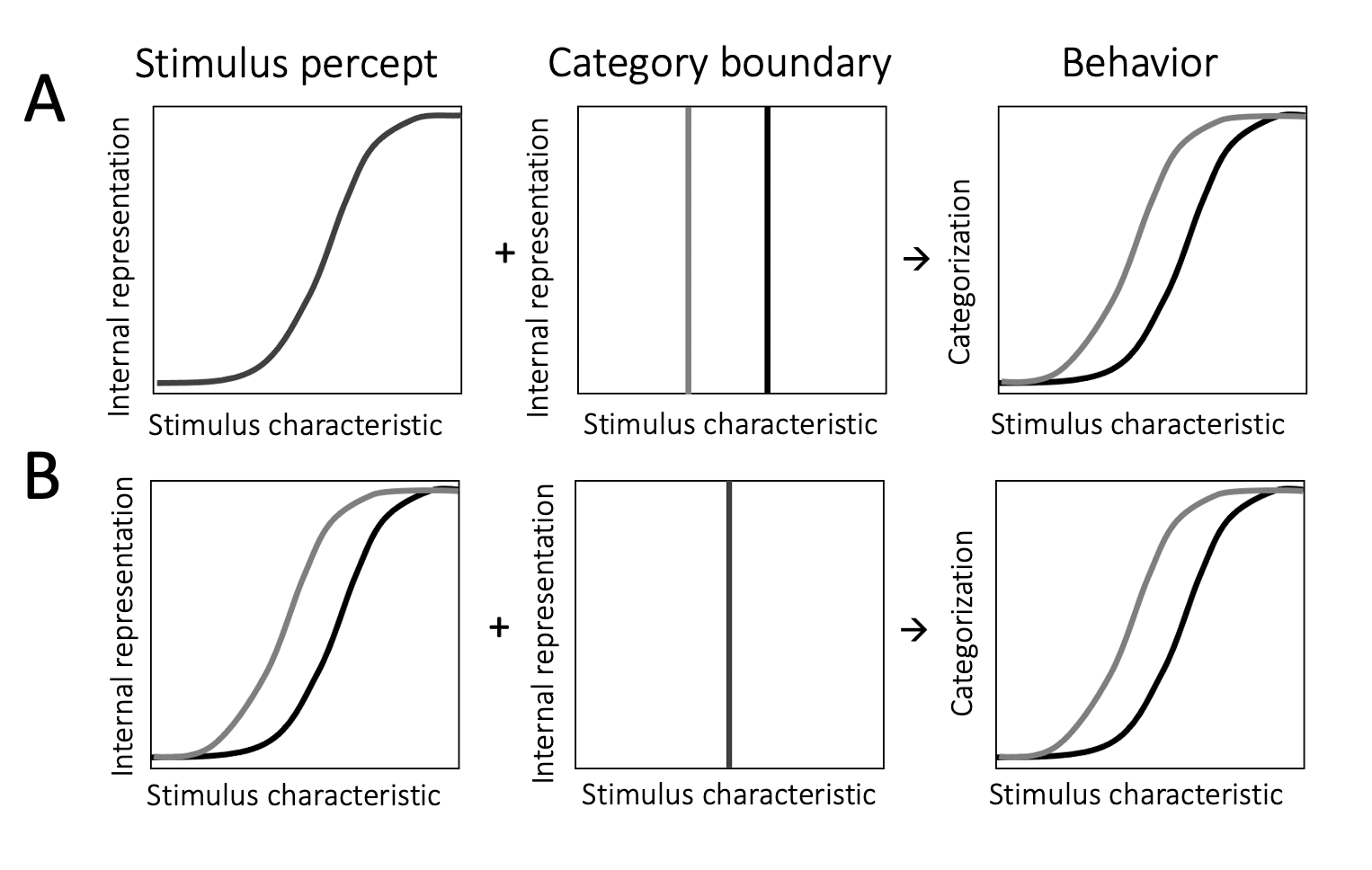
Figure 4.2: Possible sources of context dependence. \(\textbf{A:}\) Participants’ internal representation (left panel) of the stimulus is stable across contexts. Their representation of the category boundary (middle panel), however, changes such that it is lower in a context dominated by low stimulus property values (grey line) and higher in a context dominated by high stimulus property values (black line). This may be driven by a Bayesian process incorporating the prior distribution of stimulus characteristics in a noisy representation of the category boundary. It can lead to the observed context dependence in categorization decisions (right panel). \(\textbf{B:}\) Participants’ internal representation of stimulus property space shifts across contexts (left panel). This change may be driven by neural adaptation to contextual levels of stimulation. Participants’ representation of the category boundary, however, remains stable (middle panel). This can also lead to the observed context dependence in categorization decisions (right panel). Note that both of these two processes can occur at the same time and influence categorizations together.
An alternative account, popular in the literature, argues that the internal representation of the standards we use to draw category boundaries is noisy. To make categorization judgments, we draw on a working memory reference for those standards. The precision of the reference, however, decays in memory (Jou et al. 2004; Ashourian and Loewenstein 2011; Maria Olkkonen and Allred 2014). To resolve the uncertainty about its precise location in sensory (or conceptual) space, the neural system uses information available in the temporal context. It draws on the distribution of stimuli that have been recently experienced to form a prior; this prior then informs the standard. As a result, the category boundary differs across contexts – it is biased towards the central tendency of context (contraction bias), and so, behaviorally, our categorizations exhibit the observed context dependence (schematic illustration in Fig. 4.2a). A Bayesian account of this process, whereby the prior weighs more heavily in the presence of noise, is consistent with data showing that increasing the noisiness of the representation increases the contextual bias in categorizations. This can be done by, for instance, introducing cognitive demands (Ashourian and Loewenstein 2011; Allred et al. 2016) or manipulating delays between the reference and the to-be-categorized stimulus or the presentation quality of the reference (M. Olkkonen, McCarthy, and Allred 2014).
While this proposal puts the emphasis on our internal representation of the category boundary, context may also affect how we experience the current stimulus. Neural systems adapt to the levels of stimulation present in the environment. Visual adaptation to light, for instance, changes our sensitivity to stimulus brightness. After some minutes in darkness, we might be able to detect a faint light that would be indistinguishable to us in a bright room. These adaptive processes help calibrate the range of possible neural responses to the distribution of behaviorally relevant characteristics of the environment (Webster 2015) through normalization of each neural response by the pooled neural responses to context (Carandini and Heeger 2012). Adaptation can lead to changes in the appearance of stimuli, such that the neutral point (i.e. the stimulus that would be considered neutral) is shifted towards the central tendency of context. For instance, adapting to a face exhibiting an angry facial expression, would alter how we perceive subsequent faces: objectively neutral faces will cease to feel neutral and objectively angry facial expressions will appear less angry and more neutral (Webster 2011). This process may be illustrated as a recentering of the internal representation of sensory space towards the characteristics that dominate the temporal context (Fig. 4.2b). This recentering would lead to the same stimulus being encoded and experienced differently depending on the temporal context in which it is encountered. Thus, even if the internal representation of the category boundary remains stable, adaptation can capture the observed context-dependent categorization behavior.
In addition to changes to the category boundary, normalization-based adaptive processes also bring about changes in sensitivity. The sigmoid shape of the transducer function, mapping sensory space onto an internal representation, is ubiquitous in neural systems; sensitivity is highest near the inflection point of the transducer. If the transducer shifts between contexts, tracking the distribution of features, then sensitivity would necessarily change too – it would be highest for those stimulus characteristics that dominate the temporal context. Temporal context in adaptation, however, does not only encompass preceding task-relevant information. While the prior in a Bayesian process (as the one which might affect the location of the category boundary) is shaped by previously experienced instances of task-relevant stimuli, contextual influences on adaptation are less specific. Light adaptation, for instance, is driven by the overall light levels in the context, regardless of what light source is producing them (e.g. light from a lamp + moonlight = overall level of light). By contrast, our prior for the brightness of moonlight would be driven by moon brightness on previous nights, and not by our previous experiences with lamplight.
In this chapter, we set out to examine the underlying mechanisms driving context-dependent categorizations across two experiments. First, we disentangled response frequencies from the frequencies of stimulus characteristics in our contextual manipulation to rule out response bias as a driver of context-dependent categorization (Experiment 1). Second, we used the specificity of contextual influences on categorizations (Experiment 1) and changes in sensitivity (Experiment 2), to probe whether and how much adaptation contributes to the observed context dependencies across categorizations based on sensory (Experiments 1 & 2) and more abstract (Experiment 2) stimulus features.
4.2 Experiment 1
Experiment 1 measured the impact of temporal context on categorizations, controlling for biases in response frequencies introduced by the experimental manipulation. We did this by asking participants to complete one of two possible tasks on each trial. On some trials, participants had to categorize the lightness of a circle stimulus; on other trials, participants had to instead categorize its size. We manipulated the size context on trials asking about lightness categorizations only (and vice versa for lightness context manipulations). This ensured that participants were exposed to a biased set of stimulus sizes, but that they would not have to respond to disproportionately many objectively large stimuli in one context, and to disproportionately many objectively small stimuli in another. This eliminated the possibility that context-dependent categorizations could be driven by a bias, whereby participants might be striving for an equal number of “large” and “small” categorizations across contexts. At the same time, it also made it so that any such bias would act in opposition of the contextual effect. That is, in our design, responding “large” as equally often as “small” would lead to a stable categorization boundary across the different contexts, as size trials are composed of an equal number “large” and “small” ground truth categorizations in all contexts.
Experiment 1 also manipulated the timing of trials to examine two additional research questions. First, is the contextual bias in categorization decisions stronger when participants have had the opportunity to experience (and potentially, adapt to) each stimulus for longer? To address this question, we compared the contextual effect on category boundaries between a short (200ms) and long (1000ms) stimulus presentation condition. And second, how specific is the contextual effect? Is it just the context provided by task-relevant stimuli that impacts categorizations, or does the visual environment more generally also influence the location of the category boundary? The timing manipulation allowed us to examine this as participants’ visual environment, and consequently exposure to task-irrelevant properties, differed between the two stimulus timing conditions.
4.2.1 Methods
4.2.1.1 Participants
Ten participants (aged 22.3 ±4.37) with normal or corrected-to-normal vision took part in Experiment 1. The study received ethical approval from the Central University Research Ethics Committee at the University of Oxford (approval reference number: R58531/RE001) and took part in the Perception Laboratory at the Department of Experimental Psychology. All participants provided written informed consent and were compensated with either course credit or £10 per hour for their time.
4.2.1.2 Apparatus
Participants were seated in a dark room approximately 175cm away from a computer monitor (1080x1080 resolution, 32’ Display++ LCD monitor) with linearized output light intensities. Visual stimuli were created and presented with ViSaGe, CRS Toolbox (Cambridge Research Systems) for MATLAB.
4.2.1.3 Stimuli
Stimuli in the experiment consisted of grayscale circles presented on a light yellow background (CIE X=.372, Y=.400, Z=76.1\(cd/m^2\)). We followed previous work in lightness perception in choosing a chromatic background to minimize background-anchoring effects (e.g. to the minimum lightness available – black background, the maximum – white background, mean – half-contrast grey, etc.). For the contextual manipulation, we constructed 3 types of stimulus sets (low, neutral and high) for 2 stimulus property dimensions (lightness and size). For each of the two stimulus dimensions we first generated an array of 16 possible property values. Those values corresponded to the radius of the circle in pixels, and the lightness of the circle in 10-bit pixel values. We then sorted those values into two biased sets (low set: the lowest 10 values, high set: the highest 10 values) and a neutral set (the middle 10 values).
We constructed the full arrays of property values using a perceptual difference scale of lightness and size, which we estimated with a pilot group of participants (n=6, following same ethics protocol R58531/RE001) via maximum likelihood difference scaling (MLDS, Maloney and Yang 2003; Knoblauch, Maloney, et al. 2008, see Experiment 2 for details on this method). We took this approach to ensure that the stimuli we employed in the experiment would all be equally discriminable. The size array ranged from 90 to 210 pixels in steps of 8 pixels (corresponding to approximately \(1.09\)° to \(2.54\)° of visual angle at the viewing distance of the display). Note that linear step sizes in terms of radius are quadratic in terms of circle area. The lightness array ranged from 24 to 75\(cd/m^2\) in steps of 3.4\(cd/m^2\). The linear perceptual spacing of lightness we observed in piloting mirrors past results for this luminance range, (e.g. Wiebel, Aguilar, and Maertens 2017; Rogers, Knoblauch, and Franklin 2016).
4.2.1.4 Experimental Procedure
Each participant completed the experiment in a single hour-long session. The experiment consisted of 2 practice blocks and 30 test blocks of 60 trials each. Each block started with an example circle stimulus whose lightness and size corresponded to the median of the overall stimulus set. Participants were advised that they could use this circle as a reference for neutral (or medium) size and lightness.
The first practice block served to familiarize participants with the experiment. Stimuli were presented for up to 4 seconds, until a categorization response was registered. The block continued until the participant achieved an average response time of 1.5 seconds or below. The length of the first practice block was constrained to be of a minimum of 80 trials and a maximum of 150 trials. The second practice block comprised 100 trials and introduced a shorter stimulus duration – 200ms.
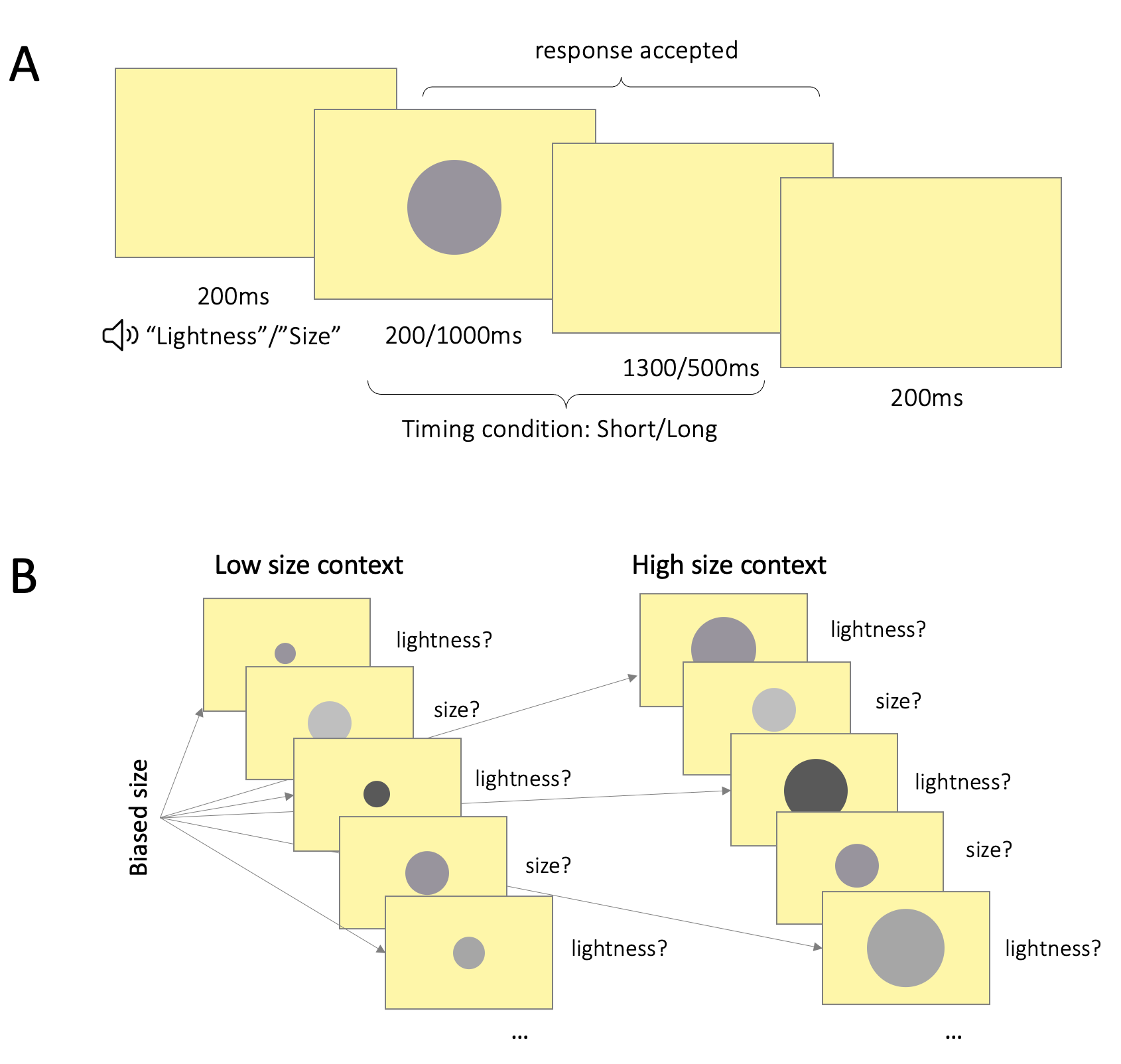
Figure 4.3: \(\textbf{A:}\) Trial structure. Participants first heard a computer generated voice announce the trial type. 200ms following this, a circle stimulus was presented in the center of the screen for either 200ms or 1000ms. In size trials, participants had to categorize the stimulus as small or large; in lightness trials, as light or dark. Responses were accepted for 1.5s starting from stimulus onset. The stimulus remained on the screen for the full stimulus duration even if the participant responded prior to stimulus offset. There were 200ms breaks between trials. \(\textbf{B:}\) Contextual manipulation. The left panel illustrates a sequence of 5 trials in a low size context, the right panel – in a high size context. Across both panels, in trials asking about size, stimulus size was drawn from a neutral set, such that half the stimuli would be objectively small and half the stimuli – objectively large. In trials asking about lightness, stimulus size was drawn from biased sets, such that stimulus size would on average be lower in the low context, and higher in the high context.
In each trial (Fig. 4.3a), the participant first heard a computer-generated voice (Google Text-to-Speech API, gender neutral voice) announce the type of trial, by producing either the word “lightness” or “size.” 200ms after the onset of the voice, a circle appeared on the screen. In size trials, participants had to categorize the circle as either large or small; in lightness trials, participants had to categorize the circle as either light or dark. Responses were accepted until the end of the trial, 1.5 seconds post stimulus onset. There was a 200ms interval between trials.
The experiment followed a 2x5 factor design. The first factor was timing – in half of the blocks, stimuli were presented for 200ms (brief condition), and in the other half of the blocks – for 1000ms (long condition). The timing manipulation allowed us to test whether the contextual effect is stronger when the participant has had the opportunity to adapt to the stimulus set for longer. That is, is there an interaction between stimulus duration and the contextual manipulation? The timing manipulation also allowed us to test another question – how specific is the contextual effect? Are categorization decisions impacted only by the context provided by previous task-relevant stimuli, or do other, task-irrelevant inputs also affect categorizations? In the brief condition, participants were exposed to the background for longer than in the long stimulus presentation condition. As the luminance of the background (76\(cd/m^2\)) was higher than that of the stimuli (24–75\(cd/m^2\)), in the brief condition, participants were exposed to a lighter visual environment compared to in the long condition. If participants’ categorization decisions were influenced by the properties of the task-relevant stimuli only, lightness categorizations should not differ between the brief and long conditions (since the relative frequencies of stimulus lightness values are matched across the long and short conditions). But if the contextual effects were driven by a more general adaptive process which is not specific to the imperative stimuli, we would expect lightness categorizations to differ between the two timing conditions (with higher thresholds in the brief condition). For size, as participants were seated in a dark room, the only obvious size reference available in the gaps between stimulus presentations was the size of the screen itself. By contrast, during stimulus presentations, the size environment included both the size of the monitor and the (relatively smaller) size of the current stimulus. Thus, the size environment was on average smaller in the long condition (where stimuli were presented for longer) that in the brief condition. We reasoned that, according to the adaptation hypothesis, this might lead to the same pattern of contextual bias for size as for lightness – higher categorization thresholds in the brief condition.
The second experimental factor was the contextual manipulation. In each block, we manipulated the context for only one stimulus dimension by using a biased set (i.e. either the low or high stimulus set) in the trials that asked about the other stimulus dimension (Fig. 4.3b). For instance, in a “high size” block, stimulus size was drawn from the high size stimulus set only on trials that asked participants to categorize the lightness of the circle; on trials where the participant had to categorize the size of the circle, stimulus size was drawn from the neutral size stimulus set. This ensured that our contextual manipulation would not introduce a confounding response bias, i.e. it would not skew the ground truth number of ‘large’ responses. In each block, we manipulated the context for only one stimulus dimension, the context for the other stimulus dimension remained neutral (neutral stimulus set). This resulted in 4 combinations of context conditions (size-lightness: high-neutral, low-neutral, neutral-high, neutral-low), to which we added a fifth neutral condition (neutral-neutral).
Responses were registered via button presses on a hand-held number keyboard. Participants were instructed to hold the keyboard with both hands and respond with their left thumb on size trials, and right thumb on lightness trials (or vice versa, counterbalanced across participants). Categorizing a stimulus as “large” or “light” was associated with the press of an upper button; categorizing a stimulus as “small” or “dark” was associated with the press of a down button. As the timings of the trials were fixed, nothing changed on the screen upon participant response; instead, participants heard a click to confirm their choice was registered.
4.2.1.5 Analyses
First, we estimated psychometric functions separately for each participant and each condition in the experiment, using the Psignifit toolbox for MATLAB (Schütt et al. 2015). We tested whether the contextual manipulation biased participants’ categorization decisions on the group level with a general linear model (GLM) of participant thresholds (normalized as a \(z\) score). The GLM quantified the impact of the contextual manipulation (coded as -1, 0, 1 for low, neutral and high), timing condition, and their interaction, controlling for the nonindependence of threshold measurements from the same observer. We followed up the results of the GLM with pairwise comparisons with paired samples \(t\) tests.
As a complementary approach for probing the effect of temporal context, we regressed participant choices on each trial on the relevant property of the stimulus on the current trial, as well as on the value of that same property on the previous 3 trials. Thus, for each participant we built two logistic regression models, one for lightness and one for size. In the model for size, the outcome variable comprised the responses to all trials asking the participant to categorize the size of the stimulus; the predictor variables included the size of the stimulus on the current trial \(t\), as well as the size of the stimuli on the immediately preceding 3 trials, \(t-1\), \(t-2\) and \(t-3\) (all predictors were \(z\)-scored). This approach allowed us to quantify the effect of stimulus history (size on previous trials, \(t-1\), \(t-2\) and \(t-3\)), controlling for the effect of the imperative stimulus (size on current trial, \(t-1\)). Note that as trial types (lightness or size categorizations) were interleaved, the predictor variables in the regression included both types of trials. For instance, in a regression on lightness categorizations, we included as predictors the lightness of stimuli on the preceding three trials; on some of those trials, the participant was likely asked to judge the size (and not lightness) of the stimulus. We assessed the statistical significance of the beta coefficients from the regression on the group level via one sample \(t\) tests.
4.2.1.6 Data & Code Availability Statement
All data and code to reproduce the analyses are available in the OSF repository (https://osf.io/vxh3n/) for this project.
4.2.2 Results
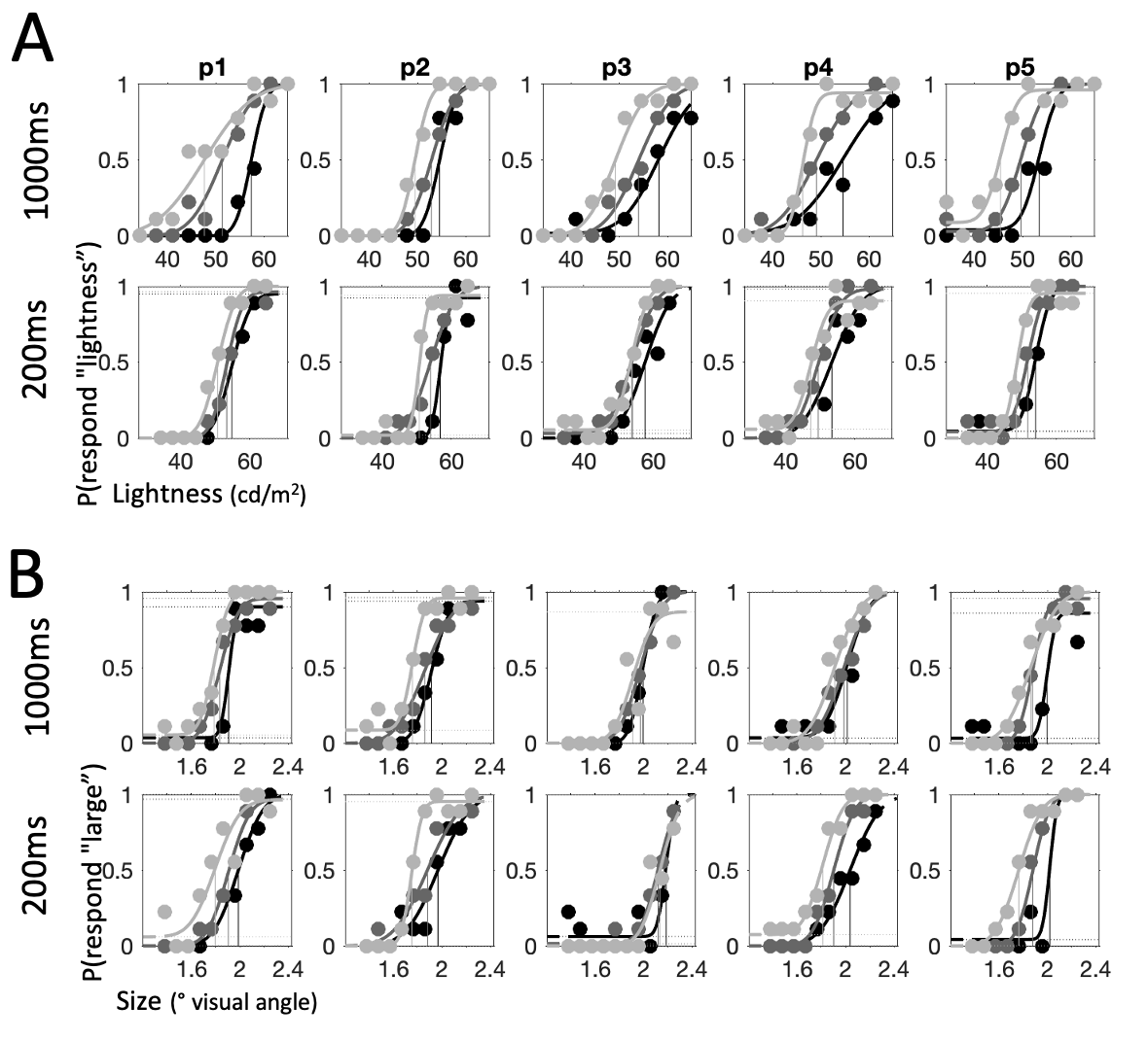
Figure 4.4: Psychometric functions for each individual participant: first half of participants, continued in the next figure. Across all panels, columns depict individual participants (p1-p10). Shading tracks context (light grey: low, dark grey: neutral, black: high). Points show raw data, curves – cumulative Gaussian functions fit to data. Vertical lines show threshold value estimates for each condition. \(\textbf{A:}\) Psychometric functions for lightness trials. Top row shows long condition (1000ms) and bottom row – short condition (200ms). \(\textbf{B:}\) Psychometric functions for size trials. Top row shows long condition (1000ms) and bottom row – short condition (200ms).
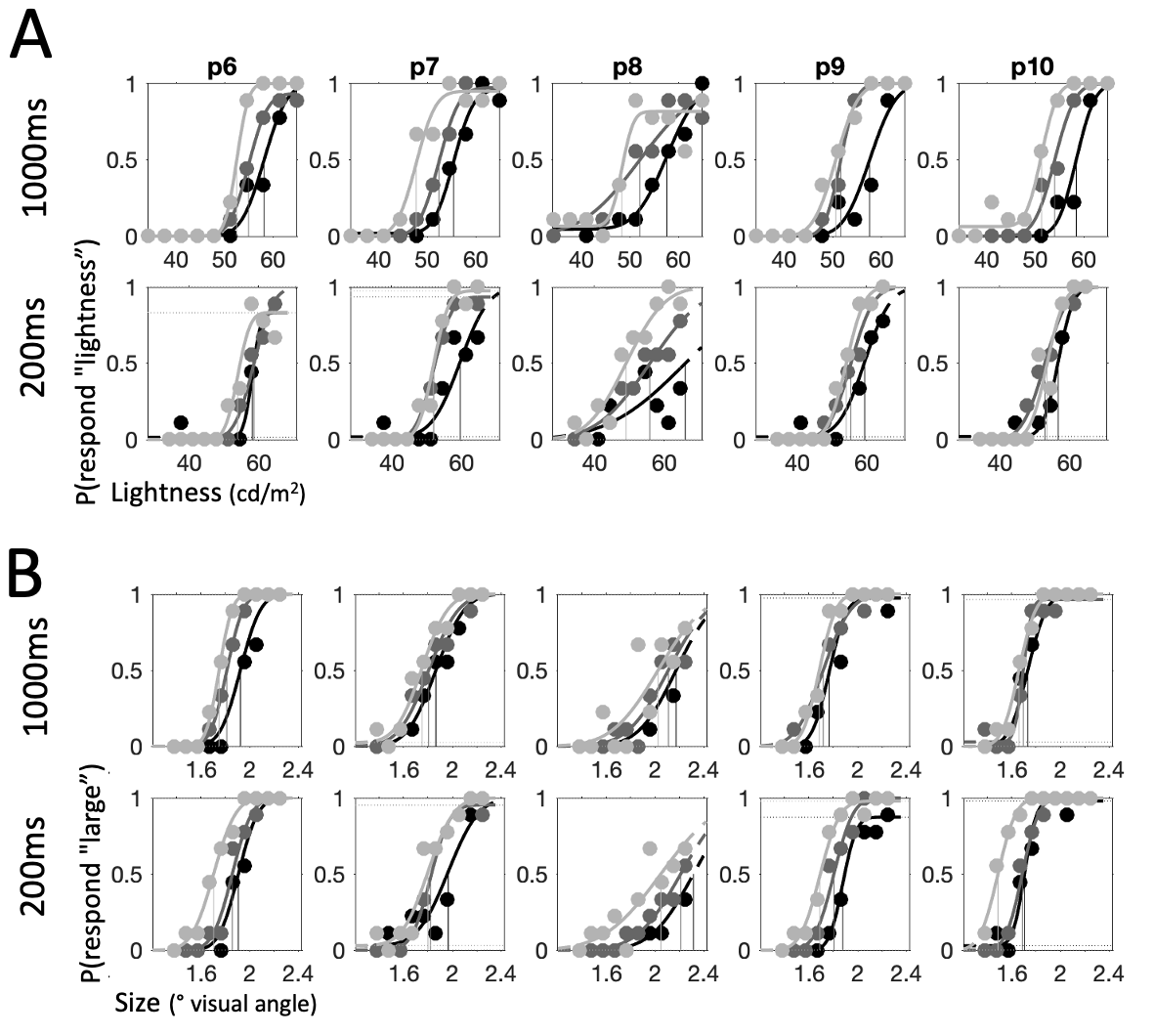
Figure 4.5: Psychometric functions for each individual participant: second half of participants, continued from previous figure
The psychometric functions for each participant are presented in Fig. 4.4 and Fig. 4.5 where each column represents one participant. While there is considerable variability in performance, there is also a clear pattern of dissociation of psychometric functions between the different context conditions. Generally, the psychometric function for the low condition (light grey) is shifted to the left and the psychometric function for the high condition (black) is shifted to the right relative to the psychometric function for the neutral condition (dark grey). These horizontal shifts in the psychometric function are captured by the parameter \(threshold\), which tracks the stimulus property value that corresponds to an equal probability of categorizing a stimulus as “large” or “small” (/“light” or “dark”). Threshold values are visualized in Fig. 4.4 as vertical lines projecting downwards from the inflection point of each psychometric function.
The average values of the thresholds across participants are presented in Fig. 4.6. We quantitatively assessed the influence of context and stimulus timing on threshold values via a GLM, controlling for individual influences on thresholds. The contextual manipulation significantly influenced categorizations (lightness: \(\beta=0.81\), \(p<0.0001\), size: \(\beta=0.63\), \(p<0.0001\)), such that thresholds increased from low to neutral, and neutral to high conditions. Pairwise comparisons confirmed this pattern of results (lightness low<neutral: \(t_9=6.78\), \(p<0.001\), lightness neutral<high: \(t_9=8.66\), \(p<0.001\); size low<neutral: \(t_9=7.02\), \(p<0.001\), size neutral<high: \(t_9=7.97\), \(p<0.001\)).
Stimulus timing impacted lightness thresholds (\(\beta=-0.45\), \(p<0.001\)), with higher thresholds for lightness judgments in the brief presentation condition. Shorter stimulus timing also increased thresholds for size judgments (\(\beta=-0.21\), \(p=0.01\)), albeit the effect was weaker than for lightness. This pattern of results suggests that categorization decisions are subject to contextual influences going beyond the immediately task-relevant stimuli. In the brief condition, the relatively high lightness of the background provided a lighter visual environment across all context conditions, resulting in higher categorization thresholds for lightness. Similarly, the brief condition provided, on average, a larger size reference, leading to increased categorization thresholds for size. This result suggests that the visual environment (beyond the immediately task-relevant inputs) contributes to the contextual bias in categorization decisions.
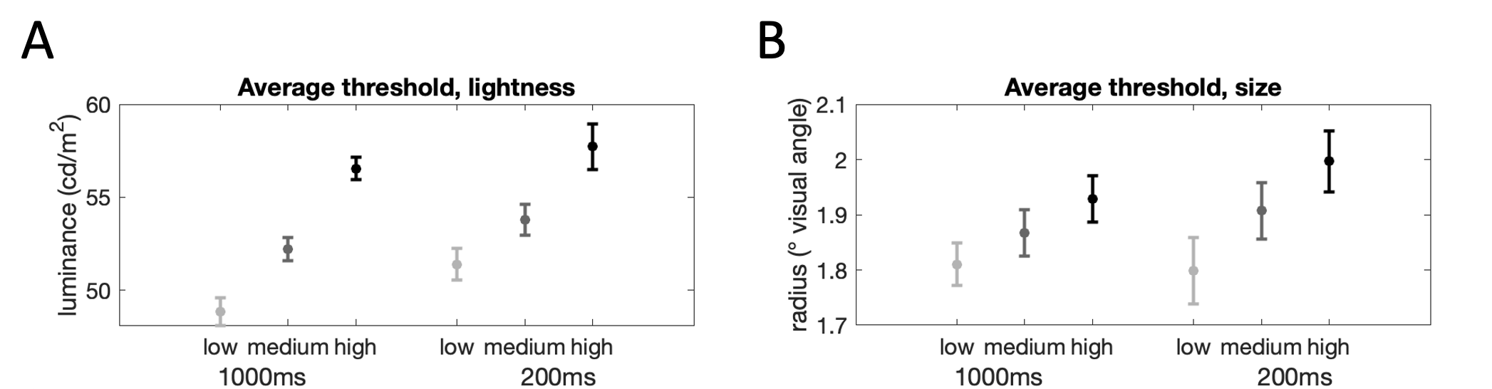
Figure 4.6: Threshold values for each context condition (light grey: low, dark grey: neutral, black: high) and timing condition (left: long, right: short). \(\textbf{A:}\) Lightness judgments. \(\textbf{B:}\) Size judgments.
Finally, the interaction between timing and context was not statistically significant for lightness (\(\beta=0.18\), \(p=0.20\)). This null result indicates that the contextual effect for lightness did not increase when participants were exposed to stimuli for longer (1000ms vs 200ms). The interaction between stimulus duration and context for size, however, was significant (\(\beta=-0.26\), \(p=0.01\)) indicating that the contextual effect decreased when participants were exposed to stimuli for longer (1000ms vs 200ms). Note that this effect goes in the opposite direction of the adaptation prediction; an adaptive process should lead to stronger context-dependencies as stimulus duration increases.
We explored the effect of temporal context further by quantifying the influences of recent stimulus history on choice via a logistic regression. The resulting beta coefficients for the decision-relevant stimulus property on the most recent 4 trials are available in Fig. 4.7. As expected, the lightness (\(t_9=14.31\), \(p<0.001\)) and size (\(t_9=14.95\), \(p<0.001\)) of the stimulus on the current trial were both strongly associated with a higher likelihood of categorizing it as light and large, respectively. Categorizations were, however, repulsed away from the properties of the stimulus on the preceding trials. Higher stimulus lightness on the previous trial(s) led to a lower likelihood of categorizing the stimulus on the current trial as light (trial \(t-1\): \(t_9=-5.00\), \(p<0.01\); trial \(t-2\): \(t_9=-10.10\), \(p<0.001\); trial \(t-3\): \(t_9=-7.24\), \(p<0.001\)). Similarly, higher stimulus size on the previous trial(s) led to a lower likelihood of categorizing the stimulus on the current trial as large (trial \(t-1\): \(t_9=-5.31\), \(p<0.001\); trial \(t-2\): \(t_9=-5.39\), \(p<0.001\); trial \(t-3\): \(t_9=-4.80\), \(p=0.001\)). Exploratory analyses (by adding more predictor variables to the logistic regression) indicated that the effect of stimulus history extended as far back as to the preceding 13 trials for lightness (trial \(t-13\): \(t_9=-3.17\), \(p=0.01\)), and the preceding 8 trials for size (trial \(t-9\): \(t_9=-4.13\), \(p<0.01\)).
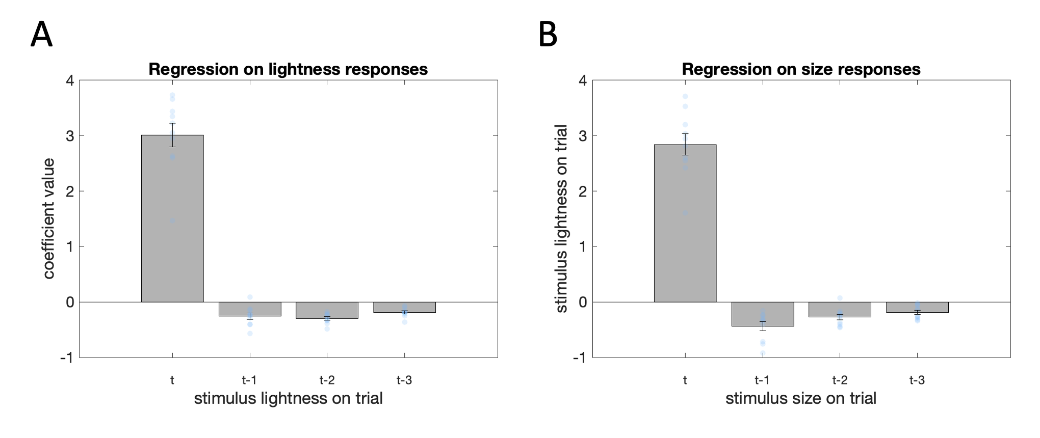
Figure 4.7: Regression on stimulus history. Across both panels, the height of the bar depicts the average standardized coefficient value for the stimulus property value on the current trial (first bar: trial t), the stimulus property value on the immediately preceding trial (second bar: trial t-1), the stimulus property value on trial before last (second bar: trial t-2), and the stimulus property value three trials ago (second bar: trial t-3). Error bars depict SEM, blue dots show coefficient values for individual participants. \(\textbf{A:}\) Coefficients for lightness responses. \(\textbf{B:}\) Coefficients for size responses.
4.2.3 Interim Discussion
Temporal context yielded a significant influence on categorizations in Experiment 1. Category boundaries for size and lightness were higher when the temporal context was dominated by larger and lighter stimuli; categorization judgments were also repulsed from the task-relevant characteristics of the stimuli on preceding trials. The smaller the size of the preceding stimuli, the more likely the current stimulus to be categorized as large. Our experimental design allowed us to rule out response bias as a driver of the observed effects. In fact, temporal context biases decisions even when this would lead to a distortion in the relative frequency of actions. This is because in our design, the relative frequency of ground truth “high” and “low” judgments was carefully counterbalanced. Thus, context-dependent categorization necessarily skews the distribution of “high” vs “low” responses.
We did not find evidence that the contextual effect increases when each stimulus is presented for 1000ms versus 200ms. We predicted that longer stimulus durations would allow for additional adaptation to the stimulus set. Contrary to our prediction, for size, we found that shorter stimulus durations led to stronger contextual biases. This finding may speak to the literature on the effect of noise on context-dependencies; shorter stimulus durations made the task more demanding. A Bayesian perspective dictates that this should lead to heavier reliance on the prior and consequently, stronger contextual biases. Interpreted in this light, our results appear to provide support for a Bayesian contraction bias mechanism driving the observed context dependence.
However, we did also find evidence that the contextual effect is not isolated to task-relevant information. Contrary to the predictions of a Bayesian process, which incorporated the distribution of recently experienced stimulus properties in a prior, we found that participants were also biased by task-irrelevant visual information. Categorization thresholds were higher in the brief condition where the task-irrelevant visual environment was lighter and larger. This suggests that a more automatic, sensory visual adaptation process, acting on our perception of the current to-be-categorized stimulus, likely contributes to the observed contextual dependencies. In Experiment 2, we follow up on these findings and assess more directly the contributions of adaptation.
4.3 Experiment 2
In Experiment 2, we aimed to disentangle the two putative sources of contextual influence – changes to our representation of the category boundary (Fig. 4.2a) versus changes to our experience of the current stimulus (Fig. 4.2b). We took advantage of the fact that adaptation processes, which impact our perception of incoming input, are characterized by changes in sensitivity to the dominating characteristics in the environment. Thus, we estimated the contribution of adaptation to context-dependent categorization judgments by comparing participants’ sensitivity to stimulus characteristics across two temporal contexts. We did this separately for the two visual properties from Experiment 1, size and lightness, as well as for a more abstract stimulus property – numerosity. Computing numerical magnitudes engages later stages of processing compared to low-level visual properties, such as lightness, contrast or orientation (Heng, Woodford, and Polania 2020) and has been linked with various higher-level cognitive processes, which rely on an ‘approximate number system’ (Piazza et al. 2007; Nieder and Dehaene 2009). Imprecision in the estimation of numerical magnitudes has also been put forth as the driver of biases in value-based decisions about economic prospects (Woodford 2020). Consequently, including numerosity in this experiment allows us to link the current chapter more closely with context dependencies in economic decisions.
4.3.1 Methods
While Experiment 1 was conducted in the Perception Laboratory at the Department of Experimental Psychology, the pandemic prevented onsite data collection for Experiment 2. Thus, all data for this experiment were collected remotely.
4.3.1.1 Participants
Twenty participants (aged 28.3 ±8.63) with normal or corrected-to-normal vision took part in Experiment 2. The study received ethical approval from the Central University Research Ethics Committee at the University of Oxford (approval reference number: R55652/RE005). All participants provided written informed consent and were compensated with £10 per hour for their time.
4.3.1.2 Aparatus
Participants completed the experiment on their personal computers. The study was programmed using PsychoPy (Peirce 2007) and PsychoJS and was hosted on Pavlovia. The output (combined RGB) light intensities of all monitors were calibrated with a perceptual calibration method (half tone pattern matching, Xiao et al. 2011) or with a photometer (ColorCal, Cambridge Research Systems). Participants were instructed to set their monitors to the lowest brightness setting and to disable any automatic brightness adjustment or light filtering applications on their computers. We chose to conduct the perceptual calibration procedure at low brightness for two reasons. First, increasing the brightness settings on a monitor, might introduce a brightness offset (i.e. requested 0% lightness does not correspond to black pixel output, but produces some light), which would render the gamma model (\(y=x^{\gamma}\)) of the electro-optical transfer function of the monitor inaccurate. Second, human visual sensitivity to changes in brightness decreases with absolute brightness levels, and so, we can minimize variability in brightness matches by conducting them at a low brightness setting. This in turn ensures that our perceptual estimate of the electro-optical transfer function of the monitor, which is based on the brightness matches, is reliable.
Viewing distance was determined individually for each participant. We asked participants to adjust the size of a rectangle on their screen to match the size of a standard bank card (Yung et al. 2015). We used the size of the rectangle in pixels to calculate the required visual distance such that 1 pixel would subtend \(57''\) of visual angle; this ensured that the size of the stimuli in visual angle would be approximately the same for all participants.
4.3.1.3 Stimuli
The experiment consisted of three parts, each of which followed the same structure, but concerned a different stimulus property – size, lightness or numerosity. In the size part of the study, the stimuli comprised grayscale circles presented against a black background. In the lightness part of the study, the stimuli comprised grayscale circles presented against a yellow background (as in Experiment 1). In the numerosity part of the study, the stimuli comprised clouds of black and white dots of varying sizes against a grey (half contrast) background. The color (white or black) was randomly selected for each dot, ensuring that the brightness of the stimulus would not be informative for the numerosity judgment. Following previous work, we also constrained the average dot radius or the total area covered by the dots to be the same across dot clouds in each trial (Izard and Dehaene 2008; Van den Berg et al. 2017; Heng, Woodford, and Polania 2020). For each trial, we randomly chose whether to hold dot radius or total area constant. This manipulation ensured that stimulus size neither on the level of individual dots nor on the level of the entire dot cloud would be informative for the numerosity judgment.
As in Experiment 1, for each of the three properties, we constructed an array of possible property values. The full arrays consisted of 10 possible values; the lowest 7 of those constituted the low stimulus set, and the highest 7 – the high stimulus set. For size, the values ranged from 69 to 195 pixels in steps of 4 (corresponding to approximately \(1.1\)° to \(3.1\)° of visual angle). For lightness, the pixel values ranged between 0.35 and 0.65 in steps of 0.033 (assuming 0-1 range on an 8-bit monitor with linearized output intensities). For numerosity, the number of dots ranged from 8 to 52 in logarithmic steps, using a multiplier of 1.232.
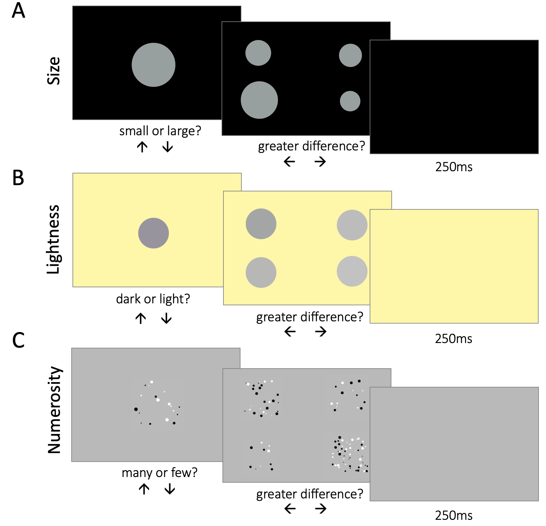
Figure 4.8: Trial structure. Across all parts of the experiment, categorization and difference comparison trials were interleaved. On categorization trials, participants saw a single stimulus in the center of the screen. On difference comparison trials, participants saw two pairs of stimuli, two stimuli on the left and two on the right size of the screen. \(\textbf{A:}\) Part 1, size task. In categorization trials, participants had to categorize circle stimuli as large or small. They responded by pressing the up or down arrow key. In difference comparison trials, participants had to compare the difference in size between the two pairs of stimuli. If they considered the difference between the stimuli on the left larger than the difference between the stimuli on the right, they responded by pressing the left arrow key (and vice versa for right). \(\textbf{B:}\) Part 2, lightness task. Participants had to categorize circle stimuli as light or dark, and compare the difference in lightness between the two pairs of stimuli. \(\textbf{C:}\) Part 3, numerosity task. Participants had to categorize clouds of dots as many or few, and compare the difference in number between the two pairs of clouds.
4.3.1.4 Experimental Procedure
The experiment took approximately 3 hours, which participants were invited to complete over three shorter sessions. Links to the online experiments are available in the OSF repository (https://osf.io/vxh3n/) for this study. We did not counterbalance the order of the parts across participants, as the subjective difficulty of the tasks in the three parts increased progressively from size through lightness to numerosity.
Across all parts of the experiment, participants had to complete two types of tasks: categorization and difference comparisons. Participants’ difference comparisons allowed us to estimate suprathreshold sensitivity. In categorization trials, participants saw a single stimulus in the center of the screen. In the size part, their task was to categorize the circle as large or small; in the lightness part – to categorize the circle as light or dark; and in the numerosity part – to categorize the number of dots in the cloud as many or few. Participants registered their choice via button press (up or down arrow). In difference comparison trials, participants saw two pairs of stimuli on the left and right side of the screen. Participants had to compare the two stimuli on the left, and decide whether the difference between them was larger than the difference between the two stimuli on the right. Thus, participants had to indicate which pair of stimuli was most different from one another. Again, they registered their choice via button press (left or right arrow). The stimuli remained on the screen for the full duration of the trial. The trial ended only when the participant provided a response.
Each part of the experiment comprised 4 blocks. Each block began with a series of 10 categorization trials, followed by 210 comparison and 210 categorization trials, presented in an interleaved fashion. We implemented the contextual manipulation during the categorization trials. In half of the blocks, the stimulus in categorization trials was drawn from the high stimulus set, and in the other half – from the low stimulus set. This resulted in two contextual bias conditions – low and high. Across all blocks, the stimuli in the difference comparison trials were drawn from the full stimulus set (i.e. the 10 value array).
4.3.1.5 Analyses
First, we analyzed categorization trials. We estimated psychometric functions for the categorization decisions of each participant for each condition (low and high context) and each stimulus type (size, lightness and numerosity). As a sanity check, we confirmed that the contextual manipulation impacted categorizations, by comparing the threshold values for the low and high context conditions via paired samples \(t\) test.
Next, we analyzed difference comparison trials. We estimated sensitivity in the two conditions via maximum likelihood difference scaling (MLDS, Maloney and Yang 2003; Knoblauch, Maloney, et al. 2008). MLDS constitutes a stochastic model of suprathreshold perceptual differences. The model assigns each of the 10 stimuli in the experiment a value on a latent perceptual scale, \(\psi_1\) to \(\psi_{10}\), such that the absolute differences between scale values (corresponding to the stimuli on a given trial) maximize the likelihood of the participant’s response (the reported difference comparison). Since any linear transformation of the perceptual scale produces the same pattern of results, the model constrains the scale to span values between 0 and 1, (i.e. \(\psi_1=0\) and \(\psi_{10}=1\)). Thus, there are 8 free \(\psi\) parameters (\(\psi_2\) to \(\psi_9\)) plus one additional free scaling term, \(\sigma\), which tracks the variability of participant responses. To assess whether the temporal context manipulation led to changes in suprathreshold sensitivity, we compared the perceptual scales estimated based on responses in the low condition (\(\psi_2^l\) to \(\psi_9^l\)) and responses in the high condition (\(\psi_2^h\) to \(\psi_9^h\)). More specifically, an adaptive process should lead to higher sensitivity for low stimulus magnitudes in the low context condition and higher sensitivity for high stimulus magnitudes a in the high context condition. We tested this prediction on the group level with a GLM, which quantified the impact of the contextual manipulation on participants’ scale values (\(\psi_{2-9}^l\) and \(\psi_{2-9}^h\)), controlling for the nonindependence of scale values from the same observer and for the effect of stimulus level (2-9). To ascertain whether the effect of context was localized to a portion of stimulus space (e.g. the lower of higher end of stimulus values), we also assessed the statistical significance and direction of the coefficient for the interaction between context and stimulus level via a GLM.
4.3.1.6 Computational Modeling
Finally, to bridge the results from categorical and difference comparison trials, we built one common model encompassing both tasks. At the heart of the model is the assumption depicted in Fig. 4.2. That is, the model assumes that categorization decisions are based on the participant’s representation of the stimulus (Fig. 4.2b) and the participant’s representation of the category boundary (Fig. 4.2a), both of which might differ between contexts: \[\begin{equation} \begin{aligned} r_{cat}^l = \frac{1}{1+\exp(-((x-c^l)-b^l) \cdot s^{-1})}\\ \\ r_{cat}^h = \frac{1}{1+\exp(-((x-c^h)-b^h) \cdot s^{-1})} \end{aligned} \end{equation}\] where \(r_{cat}\) refers to the categorization decision, which is a logistic function of the stimulus property \(x\); the superscripts \(h\) and \(l\) denote the relevant context (high and low). The model comprises 2 free parameters tracking changes to the stimulus representation (\(c^l\) and \(c^h\)), and 2 free parameters tracking changes to the category boundary (\(b^l\) and \(b^h\)). The former two parameters determine the location of the transducer function along stimulus space, the latter two free parameters determine the location of the category boundary along stimulus space. A further free parameter, \(s\), determines the slope of the transducer which may differ between participants.
If the model were fit to categorization decisions only, the parameters tracking the contextual shift in the transducer would trade off with the parameters tracking the contextual shift in category boundary, and so, it would not be possible to reliably estimate both. However, difference comparison trials are based on the participant’s representation of the stimulus only, and not on the representation of the category boundary: \[\begin{equation} \begin{aligned} y_i^l = \frac{1}{1+\exp-((x_i-c^l) \cdot s^{-1})} \\ \\ y_i^h = \frac{1}{1+\exp-((x_i-c^h) \cdot s^{-1})} \\ \\ r_{diff}^l = |y_1^l - y_2^l| - |y_3^l - y_4^l| \\ \\ r_{diff}^h = |y_1^h - y_2^h| - |y_3^h - y_4^h| \end{aligned} \end{equation}\] where \(r_{diff}\) refers to the difference comparison decision, \(y_i\) refers to the representation of stimulus \(x_i\) and the subscript \(i\) tracks each of the four stimuli on a difference comparison trial. Thus, feeding information about participants’ difference comparisons into the model allowed us to disentangle contextual changes to the representation of the stimulus (\(c^l\) versus \(c^h\)) from contextual changes to the representation of the category boundary (\(b^l\) and \(b^h\)).
We fit the model to empirical data from the experiment individually for each participant and each condition via gradient descent, implemented using the globalsearch algorithm from the MATLAB Optimization Toolbox. The best fitting parameter values allowed us to estimate the relative contributions of the two putative sources of influence to the contextual bias in categorizations. We did this by, first, calculating the contextual difference in the representation of the category boundary (\(\Delta(b)=b^h-b^l\)) and the contextual difference in the representation of the stimulus (\(\Delta(c)=c^h-c^h\)), as well as their sum (\(\Delta(total)=\Delta(b)+\Delta(c)\)); we then estimated their relative strengths (\(\frac{\Delta(c)}{\Delta(total)}\)).
4.3.1.7 Data & Code Availability Statement
All data and code to reproduce the analyses are available in the OSF repository (https://osf.io/vxh3n/) for this project.
4.3.2 Results
Psychometric functions for categorization decisions are available in Fig. 4.9a; there is clear separation between low and high context conditions. Paired samples \(t\) tests on participants’ threshold values for the two contexts confirm that categorization boundaries were higher in the high context across size (\(t_{18}=10.18\), \(p<0.0001\)), lightness (\(t_{18}=7.41\), \(p<0.0001\)), and numerosity (\(t_{18}=5.95\), \(p<0.0001\)) judgments (Fig. 4.9b). We excluded one participant from the main analyses, as visual inspection of their psychometric function indicated that they responded randomly on the categorization task for numerosity. We confirmed this by estimating the impact of the numerosity of each stimulus on that participant’s categorization judgment via logistic regression (coefficient in the low condition \(b=0.04\), \(p=0.49\), coefficient in the high condition: \(b=0.05\), \(p=0.32\)).
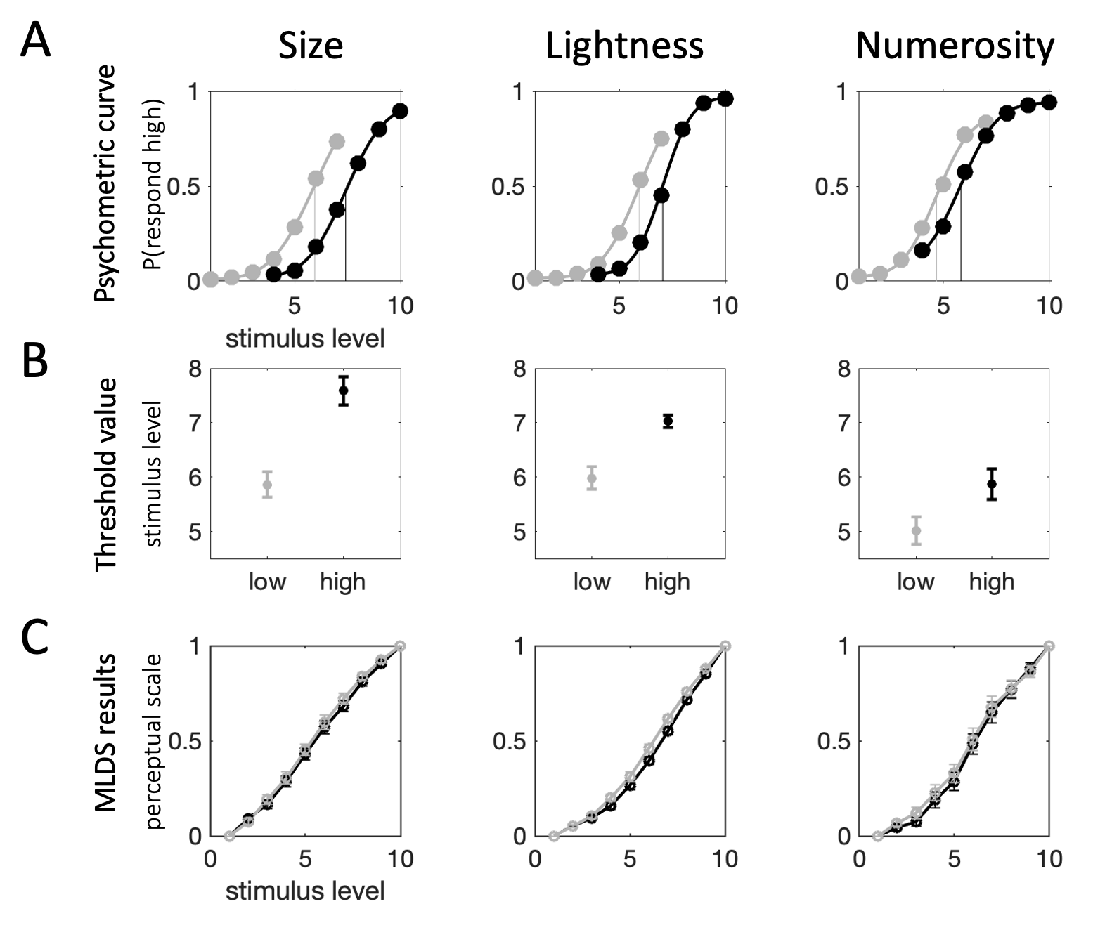
Figure 4.9: Experiment 2 results. Columns show results for each of the three different parts (left: size, middle: lightness and right: numerosity). \(\textbf{A:}\) Psychometric functions based on aggregate data collapsed across participants. Points show raw data, curves – cumulative Gaussian functions fit to data. Vertical lines show threshold value estimates for each condition. Shading indexes context condition (grey: low, black: high). Note that these average curves are for illustration purposes only, they are not necessarily representative of any one participant in the experiment. \(\textbf{B:}\) Average threshold values (across all participants) for the two conditions (grey: low, black: high). Error bars depict SEM. \(\textbf{C:}\) Perceptual scales for the two conditions (grey: low, black: high). Dots depict average scale value across participants, error bars depict SEM.
Perceptual scales estimated from participants’ difference comparison decisions are depicted in Fig. 4.9c. The plots show the average estimates of perceptual scale values of all participants, error bars track SEM, shading denotes context. The distance between scale values (on the same perceptual scale) illustrates the estimated sensitivity – the further away two points are, the more easily the participant can distinguish the stimuli they refer to. Thus, if the perceptual scale lay on the identity line (i.e. all points were equidistant along the y-axis) then all stimuli would be equally discriminable, and so, participants would be equally sensitive to changes along stimulus space. Distortions to the perceptual scale, on the other hand, illustrate differential sensitivity. For instance, the more convex the perceptual scale, the higher the relative sensitivity for higher values of the stimulus property compared to lower values of the stimulus property. This means that the directionality of the dissociation between perceptual scales in the two contexts is important. An adaptive process should lead to higher sensitivity to high stimulus property values in the high context, and to low stimulus property values in the low context. Consequently, we would expect to see a more convex perceptual scale for the high context (i.e. black curve below the grey curve).
The trends depicted by the average perceptual scales (Fig. 4.9c) seem to, on the whole, conform to this pattern. However, the effect appears small. Statistical tests confirmed that the contextual effect on sensitivity was reliable on the group level across all three stimulus types (size: \(\beta=0.10\), \(p<0.0001\), lightness: \(\beta=0.08\), \(p<0.0001\), numerosity: \(\beta=0.10\), \(p<0.0001\)). We did not find evidence that this effect was localized to the lower or higher end of stimulus space; the interaction between context and stimulus level was not statistically significant (size: \(\beta=-0.004\), \(p=0.20\), lightness: \(\beta=-0.005\), \(p=0.09\), numerosity: \(\beta=0.006\), \(p=0.22\)).
Finally, we estimated the relative contributions of the two putative sources of influence on context-dependent categorizations using our common model for the two types of tasks. Fig. 4.10 shows the results of the model fitting exercise. The three values plotted on each panel depict the average estimates for the difference in parameter values for the internal representation of the stimulus (diamond dot: \(\Delta(c) = c^h - c^l\)), the difference in parameter values for the internal representation of the category boundary (square dot: \(\Delta(b) = b^h - b^l\)), and their sum (hexagonal dot: \(\Delta(total) = \Delta(c) + \Delta(b)\)), which tracks the contextual difference in categorization behavior between the two contexts.
Generally, model estimates are consistent with the results reported above. As can be seen from the plots in Fig. 4.10, for size and numerosity, the total contextual difference in categorization judgments (\(\Delta(total)\)) was driven primarily by changes to the representation of the category boundary (\(\Delta(b)\)). On average, differences in the representation of the category boundary explained 89% and 73% of the difference in categorization judgments for size and numerosity stimuli, respectively. For lightness, changes in the representation of the category boundary (\(\Delta(b)\)) contributed approximately 54% of the difference in categorization judgments, suggesting that adaptation accounts for about half of the contextual bias in lightness categorizations.

Figure 4.10: Model results. Each panel depicts the difference in parameters between the high and low context conditions. The diamond-shaped dot corresponds to the difference between the parameters for the representation of the stimulus (\(\Delta(c)\)). The square dot corresponds to the difference between the parameters for the representation of the category boundary (\(\Delta(b)\)). The hexagonal dot corresponds to the total difference between parameters in the two conditions (\(\Delta(total)\)). Error bars track SEM. \(\textbf{A:}\) Size task. \(\textbf{B:}\) Lightness task. \(\textbf{C:}\) Numerosity task.
4.3.3 Interim Discussion
Experiment 2 also provided evidence for the robust influence of temporal context on categorization judgments. The effects held across all three properties we tested. When the context was dominated by larger, lighter and more numerous stimuli, category boundaries were pushed towards higher levels of size, lightness and numerosity. We found evidence that adaptation contributes to the observed context dependencies. On average, participants exhibited changes in sensitivity; however, those changes were modest in magnitude and differed between stimulus types. For lightness judgments, approximately half of the contextual bias can be captured by adaptation. For size and numerosity judgments, adaptation may account for 11% and 28% of the contextual bias. This pattern of results is consistent with the extensive literature on visual adaptation to light levels (Reuter 2011; Barlow 1972), and the sparser literature on adaptation to size (Blakemore and Sutton 1969; Zimmermann and Fink 2016) and higher level “cognitive adaptation” processes (Palumbo, D’Ascenzo, and Tommasi 2017). These results suggest that an adaptive encoding process adjusting the perception of a to-be-categorized stimulus contributes to the observed context dependencies in categorization.
4.4 Discussion
The temporal context in which a stimulus is situated affects how we choose to categorize it. Across two experiments, we replicate the robust contextual biases in categorization documented in the literature. When the temporal context is dominated by larger, lighter and more numerous stimuli, participants are more likely to categorize an objectively neutral stimulus as small, dark and low in number. We probed the computational origins of this bias.
The results of Experiment 1 demonstrated that context-dependent categorizations cannot be explained by a response bias driving an equal distribution of actions across contexts. Both experiments provide evidence that adaptation contributes to context dependencies in categorization decisions. Experiment 1 shows that contextual judgments are influenced by the visual environment beyond immediately task relevant inputs, consistent with the predictions of visual adaptation. Experiment 2 provides evidence that sensitivity to changes in stimulus characteristics shifts in a direction predicted by a normalization-based adaptive encoding process. The magnitude of the observed adaptation varies – it is strongest for lightness, accounting for about half of the contextual bias in categorization decisions, and more modest in magnitude but significant for size and numerosity.
This adaptation process, however, does not lead to stronger contextual biases when each stimulus is experienced for 1000ms versus 200ms. This result speaks to the rich literature on the time courses of adaptation. Visual adaptation, for instance, has been documented to occur on timescales ranging between milliseconds to years over the course of an individual’s lifetime (Webster 2015). The dynamics of adaptation in the mammalian visual system vary with the past history of stimulation; the discriminability of changes to the stimulus characteristics as well as their statistical properties can also change the observed timescale of adaptation (measured over the course of seconds and minutes, Wark, Fairhall, and Rieke 2009). It is likely that all of these factors contribute to the adaptation effects we observe here. In Experiment 1, we manipulate context on the level of an experimental block (lasting ~5 minutes), yet each stimulus is presented on the screen for a much briefer duration (\(\leq\) a second). Crucially, stimulus duration also varied on the block level, allowing the visual system to adjust to the timings of incoming stimuli and update the timescale of adaptation.
We found that shorter stimulus presentation led to more context-dependent performance for size judgments. This finding is in line with a Bayesian hypothesis (M. Olkkonen, McCarthy, and Allred 2014), where reducing the duration of the stimulus increases task demands – the participant has to remember the to-be-categorized stimulus as well as the category boundary in order to respond. This would lead participants to rely more heavily on the prior and so the contextual bias would be stronger, as in our size results. In Experiment 2, we estimated that contextual changes to the category boundary, akin to a Bayesian drift towards the stimulus characteristics dominating the temporal context, account for approximately the half of the context dependence observed in lightness judgments and the majority of the contextual influence in size and numerosity decisions.
Somewhat counter-intuitively, this Bayesian process produces an anti-Bayesian pattern of behavior. Typically, we might expect Bayesian influences on behavior to lead to judgments which are positively associated with the features present in the temporal context. In fact, this is exactly what happens in the commonly documented phenomenon of serial dependence, whereby choices concerning a typically noisy stimulus are attracted towards (or positively influenced by) the properties of the preceding stimulus (Fischer and Whitney 2014; Kiyonaga et al. 2017). This effect makes sense in our temporally autocorrelated sensory (and conceptual) environment. Input on time \(t\) is typically strongly correlated with input on time \(t-1\). For instance, visual scenes tend to be relatively stable over time, so if there is uncertainty about the identity of an input, previous stimulation would serve as a useful cue as to its identity. In the laboratory, however, trials are randomized and carefully counterbalanced, and so, any such adaptation effect would lead to suboptimal choice behavior biased towards an objectively unrelated and irrelevant stimulus on the preceding trial.
Here, we see the opposite pattern. In our experiments, categorization decisions are repulsed away from the properties of the stimuli on preceding trials (Fig. 4.7) as well as from the properties dominating the temporal context more generally (Fig. 4.6). This discrepancy in results is driven by a difference in task demands. In tasks where participants exhibit serial dependence, there is typically some uncertainty concerning the imperative stimulus – e.g. it has been presented prior to a short delay and so participants need to rely on a memory of the sensory experience, rather than on the sensory experience directly (Hollingworth 1910; Kiyonaga et al. 2017). To resolve that uncertainty, the neural system uses information from the temporal context like, for instance, the identity of the immediately preceding stimulus or some prior distribution of stimulus properties shaped by recent experience. The task we consider here is different. Participants need to categorize (or label) a stimulus that is currently available to them. Thus, there is no uncertainty about the imperative stimulus, the uncertainty lies in the category boundary – i.e. what should be the criterion for categorization? Thus, the prior distribution is incorporated in the standard against which participants judge the stimulus, and so, the observed effects on behavior are repulsive.
The reach of these context dependencies extends far beyond the laboratory. This is because we base our actions on how we evaluate or categorize a given stimulus or situation. If our judgments are affected by information in the temporal context, then so too will our actions exhibit robust context dependencies. According to behavioral ecology, context dependence in judgments relating to sustenance maximizes an organism’s chance for survival (Stephens and Krebs 1986; Kolling et al. 2012). When deciding whether to stick to the current resource or forage for something better, it only makes sense to expend valuable energy on foraging if it is likely that better resources would be available in the environment. Thus, our definition of an acceptable banana should change depending on context. If the available bananas are predominantly unripe, we might happily eat a banana that is a bit on the green side. Conversely, a spotted, overripe banana might make the cut in a context dominated by rotting, brown bananas.
Context, however, impacts our judgments far beyond these evolutionarily relevant realms where context dependence may serve an adaptive, fitness-maximizing purpose. For instance, an ethics review committee should maintain stable standards for the ethicality of research proposals. Yet, we know that when student volunteers are faced with this task, their decisions to accept or reject a research proposal are significantly impacted by the levels of ethicality currently dominating the context (Levari et al. 2018). In the realm of political science, the context dependence of human judgment is encapsulated in the Overton window, a term coined in the 1990s by political commentator Joseph Overton. It refers to the range of ideas that are acceptable to the public, and it can shift and expand with the evolution of public opinion. Recently, analyses have highlighted how manipulating what information dominates the public sphere can be used to alter what the general public considers acceptable (Greenhill 2018; Bobric 2021). Research into the mechanisms underlying the context dependence of human judgments, such as our study described here, bears implications for this line of work. Cognitive neuroscience can help inform the social sciences about when and how context affects behavior and what can be done to counteract it.
4.5 Conclusion
Context consistently sways categorization decisions across perception, cognition and economics. This chapter examined the computational mechanisms underlying this effect. We found that context dependencies in categorization behavior cannot be explained by a response bias, aiming to maintain the distribution of actions stable across contexts. Instead, our results suggest that context dependencies are driven by a combination of two complementary processes. The first process affects our representation of the category boundary, pushing it towards the central tendency of the context (Bayesian contraction bias). The second process affects our perception of the to-be-categorized stimulus, repelling it away from the properties of temporal context (adaptation). These two processes appear to contribute equally to the context dependence of lightness categorizations; however, the role of adaptation is weaker, yet significant, for judgments of stimulus size and numerosity.