3 How do perceptual distractors distract?

When a target stimulus occurs in the presence of distractors, decisions are less accurate. But how exactly do distractors affect choices? This chapter explores that question using measurement of human behavior, psychophysical reverse correlation and computational modeling. We contrasted two models: one in which targets and distractors have an independent influence on choices (independent model) and one in which distractors modulate choices in a way that depends on their similarity to the target (interaction model). Across three experiments, participants were asked to make fine orientation judgments about the tilt of a target grating presented adjacent to an irrelevant distractor. We found strong evidence for the interaction model, in that decisions were more sensitive when target and distractor were consistent relative to when they were inconsistent. This consistency bias occurred in the frame of reference of the decision, that is, it operated on decision values rather than on sensory signals. Further, it was independent of spatial attention. A normalization framework, where target features are normalized by the expectation and variability of the spatial context, successfully captures the observed pattern of results.

3.1 Introduction

Visual scenes in the real world are typically cluttered, and so perceptual decisions necessarily occur in the context of irrelevant information. For instance, when adjusting a crooked picture frame, a decision maker must focus on its offset from vertical, ignoring the tilts of surrounding paintings, as those are irrelevant to the task. A long line of research across psychology and neuroscience has investigated humans’ ability to focus on an imperative stimulus in the context of distracting input. A classic laboratory analogy of the above scenario asks participants to judge a cued item in a multi-element array. For example, participants might be asked to discriminate the tilt of a (cued) target grating presented among one or more irrelevant gratings (distractors). Empirical work has focused on understanding how the cue impacts behavior and modulates neural signals, informing models of how target processing is prioritized in the face of distraction (Reynolds and Chelazzi 2004; Carrasco 2011). These models have, for example, produced detailed predictions about how tuning functions in visual neurons vary according to whether the neuron’s preferred stimulus is attended or unattended (Moran and Desimone 1985; McAdams and Maunsell 1999; Treue and Trujillo 1999; Reynolds and Heeger 2009).

However, we know remarkably little about how distraction itself influences decisions. When (a cued) target and (an uncued) distractor occur together, how exactly does the distractor affect choices? This question lies at the intersection of several distinct literatures in psychology and neuroscience which are rarely discussed together. Firstly, it is sometimes argued the effects of spatial cueing can be understood through the normative lens provided by Bayesian inference. The cue provides probabilistic information about which of two locations is decision-relevant; an ideal observer will combine this with noisy signals arising from target and distractor locations, weighted by their likelihoods (according to the probabilistic cue, Dayan and Zemel 1999; Eckstein et al. 2009). In other words, the distractor and target hold independent sway over decisions, with the job of the observer being to weigh them appropriately according to prior information. Similar models have sometimes tried to subsume the literature on attention within the normative framework given by decision theory (Anderson 2011).

A related view of distraction can also be found in a popular theoretical framework proposing that stimuli effectively compete for neural resources. Attention serves as controller that can bias processing towards percepts which are more relevant for ongoing behaviors (Desimone and Duncan 1995). While this view does not clearly translate onto decision theory, it nevertheless implies that decision variables are derived from admixtures of independent (relevant and irrelevant) sensory signals, with their relative weighing determined by the strength of control, for example arising in prefrontal cortex (Miller and Cohen 2001; Egner and Hirsch 2005). Alternative but related views posit that relevant and irrelevant features race independently to drive decisions (Bundesen 1990) or contribute to the differential weighing of mutually inhibitory sources of evidence in an accumulation-to-bound model, a framework known as decision field theory (Busemeyer and Townsend 1993). One specific instance of this class of theory argues that when humans choose between a preferred and a less preferred item, inputs to the decision process are given by a subtractive mixture of the two stimulus values, with a higher weight given to the currently fixated item (Krajbich, Armel, and Rangel 2010).

What the aforementioned models share is the central idea that target and distractor contribute independently to choice. Broadly, we can view decisions as driven by a process such as: \[\begin{equation} y^{ind} = \beta_0 + \beta_1\theta_T + \beta_2\theta_D + \epsilon \end{equation}\] where \(y^{ind}\) is the decision variable, \(\theta_T\) and \(\theta_D\) are the features of the target and distractor respectively, \(\beta_1\) and \(\beta_2\) are their respective weights, and \(\epsilon\) is an error term. We can consider the application of the weights to be outside voluntary control, so that distraction is at least in part inevitable. Here, we call this the “independent” model of distraction. For the most part, assuming that accuracy is above chance, we can expect \(\beta_1>\beta_2\). Some theories posit special downstream mechanisms that attempt to eliminate the effect of \(\beta_2\) altogether, known as distractor suppression (Geng 2014; Chelazzi et al. 2019).

However, a different proposal is that target and distractor do not wield independent sway over \(y\) but rather: \[\begin{equation} y^{int} = \beta_0 + \beta_1\theta_T + \beta_2\cdot f(\theta_T|\theta_D) + \epsilon \end{equation}\] We use the term \(f(\theta_T|\theta_D)\) in this equation to refer to some unspecified process by which target and distractor interact. For instance, this could be a straightforward multiplicative process or it could involve rectification or discretization operations; e.g. target processing could be stronger or weaker when the distractor is similar/dissimilar (Blakemore, Carpenter, and Georgeson 1970) or congruent/incongruent (Eriksen and Eriksen 1974). Importantly, what this implies is that the influence of the distractor on the decision occurs only by virtue of how the distractor modulates or interacts with the target. Thus, we call this the “interaction” model of distraction.

This class of model has also been popular at various times and in various guises. For instance, one well-known body of literature discusses the phenomenon of contextual facilitation, whereby in the extrastriate visual cortex, neuronal responses to the receptive field center are biased by stimulation of the surround (Krause and Pack 2014). At the neural level, this area has been amply explored but fewer studies have examined how spatial context may modulate behavior. Still, previous work has established that detection thresholds for a grating are lowered if it is flanked by collinear gratings (U. Polat and Sagi 1994; Kapadia et al. 1995; Ito and Gilbert 1999; C. D. Gilbert and Li 2013). Here, the distractors influence the decision by virtue of their similarity to the target. Another example involving visual stimuli is the tilt illusion whereby the tilt of a central grating is perceived as repulsed away from a ring of flanking distractors (Blakemore, Carpenter, and Georgeson 1970). Again, the distractors do not influence the decision directly; for instance, decisions about the target are less repulsed if the distractors are more dissimilar, contrary to the predictions of the independent model. These sensory level interaction effects have been successfully modeled in a divisive normalization framework, where individual neural responses are scaled by the population response (Carandini and Heeger 2012).

Indeed, the family of normalization models discussed in the previous chapter, which successfully capture decoy effects in decisions about economic prospects, also constitute specific instances of the interactive model. In this class of models, known as divisive normalization, \(f(\theta_T|\theta_D)\) may be viewed as a divisive operation, following the general form \(y \sim \frac{\theta_T}{r+\theta_T+\theta_D}\), where \(r\) is a regularizer (Louie, Khaw, and Glimcher 2013; Landry and Webb 2021). Through the years, alternative explanations of the phenomenon have sometimes instead appealed to the independent account (Busemeyer and Townsend 1993). However, it is difficult to reconcile those theories with findings that the modulation strength of a decoy depends on its proximity in conceptual space to the target (Soltani, De Martino, and Camerer 2012; Landry and Webb 2021), echoing results from the perceptual literature about the effect of target-distractor similarity on choice.

Relatedly, in the cognitive domain, perception of quantities (e.g. the number of African nations) or value (the price of bottle of wine) can be anchored by irrelevant prior information (Ariely, Loewenstein, and Prelec 2003). However, anchoring by an irrelevant quantity also seems to diminish with distance between the anchor and the target value (Wegener et al. 2001), indicative of an interaction between target and distractors. Together, these effects from diverse literatures imply a view whereby distractors and targets interact. Indeed, a recent paper showed how a version of the interaction model can explain a range of distractor-mediated phenomena in perceptual, cognitive, and value-based decision tasks (V. Li et al. 2018).

This chapter describes three experiments in which participants made a fine discrimination judgement about a target grating that is presented concurrently with an irrelevant distractor grating. We combined computational modeling and reverse correlation analysis to probe how the distractor influences choices. This approach allowed us to directly compare variants of the independent and interaction models as explanations of our data. Our experiments addressed three related questions. Firstly, how does the distractor influence decisions? Secondly, does it do so at the perceptual or decision level? And thirdly, how does spatial attention mitigate (or otherwise) the effect of distraction?

3.2 Experiment 1

To investigate the influence distractors wielded on choice, we presented participants with brief flashes of a pair of Gabor patches embedded in smoothed noise. We analyzed participants’ reports of the tilt of the target grating on each trial, using information about the features of the orientation signal of both target and distractor stimuli, as well as information about the signal-like fluctuations in the noise of each stimulus.

3.2.1 Methods

3.2.1.1 Participants

Twenty-six participants (aged 25.33 ±4.38) took part in Experiment 1. Two participants were excluded from the main analyses as the accuracy of their responses for one of the possible stimulus locations was at chance level (|accuracy - 50%|<5%). Our exclusion strategy took into account that 75% accuracy (the staircase target and approximately the average performance in the experiment) could be achieved if participants only focused on one side of the screen (and achieved near 100% accuracy for stimuli there) while guessing on the other side (achieving near 50% accuracy for stimuli there). To ensure that such a strategy was not driving the observed level of accuracy, we excluded participants who performed at chance level for stimuli on either side of the screen. The study received ethical approval from the Central University Research Ethics Committee at the University of Oxford (approval reference number: R51752/RE001). All participants provided written informed consent and were compensated £10 per hour for their time.

3.2.1.2 Apparatus

Participants were seated in a dark room approximately 60cm away from a computer monitor (120Hz refresh rate, 1280x1024 resolution, 21’ CRT) with linearized output light intensities. Visual stimuli were created and presented with Psychophysics Toolbox Version 3 (PsychToolbox-3, Brainard 1997) for MATLAB.

3.2.1.3 Stimuli

The experimental stimuli were noisy gratings, each of which consisted of a Gabor pattern and smoothed Gaussian noise. The Gaussian envelope of the Gabor patterns had a standard deviation of 1° of visual angle. The phase of each Gabor pattern was sampled from a uniform distribution; orientation was drawn from a uniform distribution with range –10° to 10° rotation from a vertical decision boundary. Noise was generated independently for each stimulus by sampling pixel values from a Gaussian distribution and passing the resulting pixel values through a smoothing Gaussian filter. The dimension of the filter, 0.083° of visual angle, was chosen to maximize the trial-to-trial variability of the convolution between the smoothed noise and Gabor signal (Wyart, Nobre, and Summerfield 2012). Stimuli were presented at full contrast. The ratio of the contrast of the Gabor pattern to the contrast of the noise of a stimulus was adaptively determined for each participant (see procedure for staircase details). The average value of the contrast ratio produced by the staircase across participants was 0.35 (i.e. 35% of the contrast of the stimulus was dedicated to the signal and 65% to the smoothed noise). Stimulus size spanned 4° visual angle and stimulus position was centered at 4° of visual angle to the left and right of fixation.

3.2.1.4 Experimental Procedure

Each participant completed the experiment in a single hour-long session. The experimental session consisted of 2 training blocks and up to 9 test blocks (100 trials each). The training blocks served to familiarize participants with the task and calibrate participant performance. To this end, during training we employed an adaptive staircase procedure, accelerated stochastic approximation (Lu and Dosher 2013), to titrate the contrast ratio for the noise in the stimuli for a target participant performance of 75% correct. The training and test trials followed the same structure; the only difference was in the contrast ratio of the stimuli. During training blocks, the contrast ratio was adjusted in each trial according to the staircase, which varied the step size of the change in contrast adaptively after each response. The training blocks had a variable trial count. Each training block ended after the staircase converged and took on average between 5-10 minutes. We used the contrast ratio estimate from the second training block to generate stimuli for the test blocks.

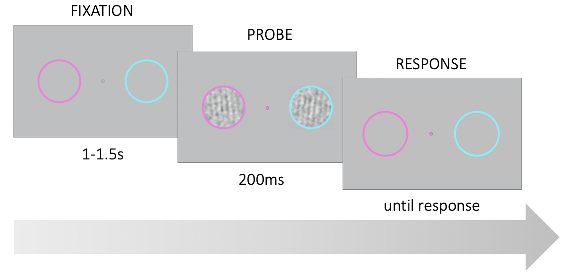
Figure 3.1: Trial structure. Participants were asked to fixate on a point in the center of the screen. Two noisy gratings appeared briefly within the colored rings on the left and right of the fixation point. At stimulus onset, the fixation point changed color and served as a probe. Participants had to report the tilt (CW or CCW) of the probed grating relative to vertical.

Each test block lasted approximately 5 minutes and participants were invited to take short breaks between blocks. During the experiment, participants were asked to fixate their gaze at the center of the screen on a fixation point between two colored rings (Fig. 3.1). The rings were located at 4° of visual angle to the left and right of center. The left ring was magenta and the right ring was cyan. In each trial, after a uniformly variable interval between 1-1.5s, two noisy gratings appeared within the colored rings for 200ms. At stimulus onset, the fixation point assumed the color of one of the two rings until the end of the trial. The color of the fixation point served as the probe indicating which of the two stimuli was the target. Participants had to report whether the target was tilted clockwise or counterclockwise (CW or CCW) relative to a vertical decision boundary. Participants reported their responses via keyboard presses (left and right arrow keys) and instantaneously received fully informative auditory feedback (correct: a high 880Hz tone, incorrect: a low 440 Hz tone).

3.2.1.5 Analyses

In our analyses, we asked how the distractor stimulus affects participant choices. We addressed this question with both regression-based and reverse correlation analytic approaches.

3.2.1.5.1 Stepwise Regression

We first took a regression-based approach to identify the contributions of the target and distractor to choice. We defined the decision-relevant features of the target \(\theta_T\) and distractor \(\theta_D\) as their respective angular offsets from the decision boundary on each trial. We assumed that choice probabilities were a logistic function of a decision variable \(y\), computed from both target and distractor features: \[\begin{equation} p(CW) = \frac{1}{1+e^{-y}} \tag{3.1} \end{equation}\] where \(p(CW)\) corresponds to the probability to respond clockwise on a given trial.

In order to ascertain the nature of the relationship between distractor features and choice, we utilized a forward and backwards stepwise regression approach for including predictors. Due to the way we have framed the question above, there is some liberty in specifying the nature of the target-distractor interaction. The hierarchical factor knock-in and knock-out approach of the stepwise regression allowed us to consider a number of possible definitions of the interactive relationship \(f(\theta_T|\theta_D)\) and empirically evaluate each of them. The predictor variables we considered included:

• \(\theta_T\), the independent effect of the target angular offset
• \(\theta_D\), the independent effect of the distractor angular offset
• \(|\theta_D|\), the absolute value of the distractor angular offset
• \(congruency\), a binary indicator whether the angular offsets of the target and distractor fall on the same side of the category boundary
• \(\theta_T \cdot \theta_D\), the (unsigned) multiplicative interaction between the target and distractor angular offsets
• \(\theta_T \cdot |\theta_D|\), the multiplicative interaction between the target angular offset and the absolute value of the distractor angular offsets
• \(\theta_T \cdot |\theta_T - \theta_D|\), the interaction between target angular offset and the consistency between the target and the distractor angular offsets

We estimated separate models for each individual participant. We used the stepwise algorithm from the MATLAB Statistics and Machine Learning Toolbox for the backward and forwards stepwise regression analysis and the Statistical Parametric Mapping Toolbox for Bayesian model selection. We used Bayesian model selection (Stephan et al. 2009) to compare the cross-validated log likelihoods of the model identified with the stepwise regression against nested competitor models.

To further explore the effect of the distractor on choices, we used logistic regression to estimate target sensitivity across different values of the distractor. We sorted distractors into 6 bins, each bin spanning 3.33°, and regressed choices within each distractor bin on target offset, \(\theta_T\): \[\begin{equation} y = \beta_0 + \beta_1\theta_T \end{equation}\]

Running this regression model separately for each distractor bin allowed us to estimate the influence of \(\theta_T\) given different values for \(\theta_D\) and detect distractor-dependent changes to target sensitivity.

3.2.1.5.2 Reverse Correlation

The regression analysis describes each target and distractor with a scalar quantity that indexes the disparity between its orientation signal and the boundary. However, the target and distractor stimuli constituted images containing multidimensional information about a full range of orientations. In particular, the energy at each orientation varied from trial to trial for both target and distractor because of the smoothed noise we applied. This allowed us to carry out a reverse correlation analysis to examine how the signal-like fluctuations in signal energy at each orientation influence choices, and thus to plot decision kernels in orientation space for both target and distractor.

3.2.1.5.2.1 Stimulus Energy Profiles

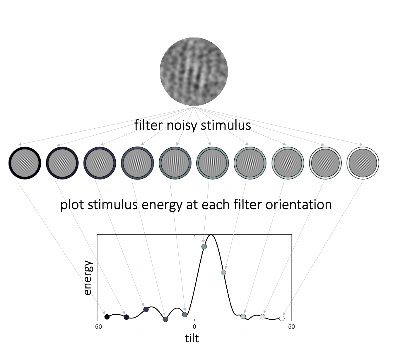
Figure 3.2: Stimulus energy profiles. We filtered each noisy stimulus through a pool of oriented Gabor patches to calculate energy across orientation space. The higher the stimulus energy at a given orientation, the more the noisy stimulus resembles a Gabor patch of that orientation. The collection of energies of a given stimulus across orientation space constitutes the energy profile of that stimulus.

To quantify the relationship between trial-to-trial signal-like fluctuations in the noise of each stimulus and participant decisions, we first characterized the filter energy of each stimulus \(S\) across orientation space using an ordered set of Gabor filters \(F^{\theta}_{\phi_n}\) (Fig. 3.2). The spatial frequency of the filters matched the spatial frequency of the Gabor patterns. Filter orientation (\({\theta}\)) ranged between -45° and 45° in increments of .5°. To correct for differences between the phase of the stimuli (sampled uniformly between \([0,1] \cdot 2\pi\)) and the filters, we specified 5 filter phases \({\phi_n}\) (\([0.1,0.9] \cdot 2\pi\), in steps of \(0.2 \cdot 2\pi\)). We calculated stimulus response to each filter \(R(S|F^{\theta}_{\phi_n})\) as the amount of variance in the filter that was explained by the covariance of the filter and stimulus. We then estimated the filter phase \(\phi^{max}\) (which can take any value between \([0,1] \cdot 2\pi\)) at which the highest response would be obtained for that orientation, by fitting the following mathematical model: \[\begin{equation} R(S|F_n^{\theta}) = E(S|\theta) \cdot \cos(\phi_n - \phi^{max}) \end{equation}\] where \(E(S|\theta)\) corresponds to the energy of the stimulus \(S\) at orientation \(\theta\), and \(\phi_n\) to the phase of filter \(n\) (\(n\) ranges from 1 to 5). Thus, the model assumes that the relationship between filter response and filter phase follows a cosine function. We can use gradient descent to identify the value of \(\phi^{max}\) that would produce the strongest filter response, as well as predict the magnitude of that response, i.e. signal energy at that orientation, \(E(S|\theta)\).

Calculating the energy profiles in this manner, that is, via convolution with Gabor filters of the same parametric specification as the target signal, ensures that we are obtaining orientation energy at the spatial scale of the target. This operation is more specific than, for instance, a Fourier transform in that it takes into account the expectation for the target (and distractor) signals. Thus, the energy profile lends itself to an intuitive interpretation – the more a noisy stimulus resembles a signal grating with a given orientation, the higher the filter energy of the stimulus at that orientation.

3.2.1.5.2.2 Decision Kernels

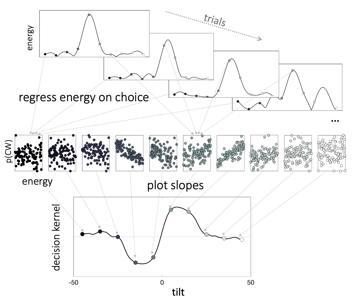
Figure 3.3: Decision kernels. We regressed choices (\(p(CW)\)) on \(z\)-scored stimulus energy via separate binomial regressions in each orientation bin. The resulting beta coefficients make up the decision kernel. Thus, the decision kernel indexes the relationship between energy at a given orientation and choice. Positive kernel values suggest that the more a stimulus resembles a Gabor patch of that orientation, the more likely is a participant to make a clockwise choice.

Next, we related fluctuations in energy at each orientation in each trial to participant choices to calculate the decision kernel, i.e. estimate of the latent function mapping stimulus features on choice (Fig. 3.3). We did this via a series of parallel binomial regressions, one per each filter orientation, with participant choice (CW or CCW) as the outcome variable and target energy \(E(T_i|\theta)\), standardized within each orientation bin as a \(z\) score, as the predictor variable. The resulting beta coefficients capture the relationship between choice and energy at each orientation, and when plotted together constitute the decision kernel. The reverse correlation approach we describe has been used previously to investigate the effects of feature expectation and attention, as well as spatial attention to target stimuli on choice sensitivity (Wyart, Nobre, and Summerfield 2012; Barbot, Wyart, and Carrasco 2014; Cheadle et al. 2015).

In addition to the kernel quantifying the relationship between target energy and choice, we calculated a kernel quantifying the direct effect of the distractor energy on choice (as in the independent model). We estimated the distractor influence by adding distractor energy as a competitive regressor in the model above. We assessed the independent effect of the distractor on choices by testing whether the average absolute values of the distractor kernel deviate from zero at different angles relative to the category boundary. To reduce the number of multiple comparisons, we divided orientation space into angles near the decision boundary (\(|\theta|<22.5\)°) and angles far from the boundary (\(|\theta|>22.5\)°) and averaged the absolute value of the decision kernel within those two bins. Our choice of median split of orientation space was guided by simulations of the theoretical decision kernels (i.e. simulated responses based on ground truth tilt corrupted by Gaussian noise). We compared the resulting kernel values in the two bins across participants to zero via a single sample \(t\) test.

3.2.1.5.2.3 Kernel Decomposition

The decision kernel is smooth, so statistical tests conducted at different orientation bins are not independent. To tackle this issue, we reduced the dimensionality of the data via singular value decomposition (SVD). This approach allowed us to derive a set of basis functions (components) from the data itself, and to assess their relative weighing in driving choices. We carried out SVD on a matrix containing the energy profiles of all stimuli, both targets and distractors, from the experiment. The rows of the matrix indexed individual stimuli and the columns indexed orientation bins. The SVD analysis produced a set of components and assigned component scores for each stimulus, which correspond to the variance in the stimulus explained by a given component.

Next, we identified the (number of) components \(V^i\) which explained 95% of the variance in the data and assessed which of them contained information about the tilt of the stimulus relative the decision boundary via visual inspection. We then used the component scores \(U^i\) for the tilt-informative component(s) of the target and distractor stimuli as predictor variables in a regression model. The model was analogous to the regression model identified through the stepwise algorithm. The only difference was that we used the component scores for the target \(U_T^i\) and distractor \(U_D^i\) instead of their angular offsets, \(\theta_T\) and \(\theta_D\), as predictor variables.

3.2.1.6 Data & Code Availability Statement

All data and code to reproduce the analyses are available in the OSF repository (https://osf.io/54rf2/) for this project.

3.2.2 Results

3.2.2.1 Regression Results

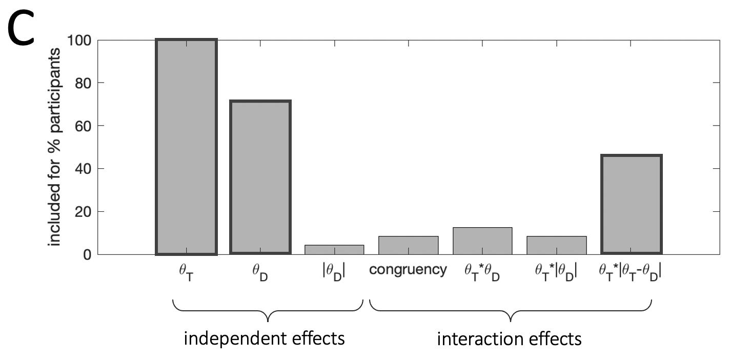
Figure 3.4: Results from stepwise regressions estimated individually for each participant in the experiment. Bar height indicates the percentage of participants for whom a parameter was included in the final model. Darker bar outlines indicate predictors we included in the final model.

Fig. 3.4 illustrates the proportion of participants whose data was best explained by a model including each of the predictor variables we considered. The model variant that best fit the human data among the candidates we considered was the following: \[\begin{equation} y = \beta_0 + \beta_1\theta_T + \beta_2\theta_D + \beta_3(\theta_T\cdot|\theta_T-\theta_D|) \tag{3.2} \end{equation}\]

This model provided a better explanation of human choices compared to models that included a different functional form for the interaction \(f(\theta_T|\theta_D)\). It also provided a better fit to models that omitted either the independent \(\theta_D\) or interaction effect \(f(\theta_T|\theta_D)\) of the distractor. Bayesian model selection on cross-validated model log likelihoods produced exceedance probabilities of \(p=0.80\) and \(p=0.99\) for this model over an independent effect only model (i.e. \(\beta_3=0\)) and over an interaction effect only model (i.e. \(\beta_2=0\)), respectively.

In Eq. (3.2) the coefficients \(\beta_1\) and \(\beta_2\) encode the influence (weight) of the target and distractor on choice. The third coefficient \(\beta_3\) encodes the influence of the target-distractor interaction. The functional form of the interaction term indicates a consistency bias – the influence of the target on choices depends on the degree of consistency between the target and distractor features. That is, choice sensitivity to \(\theta_T\) varies with the similarity between \(\theta_T\) and \(\theta_D\).

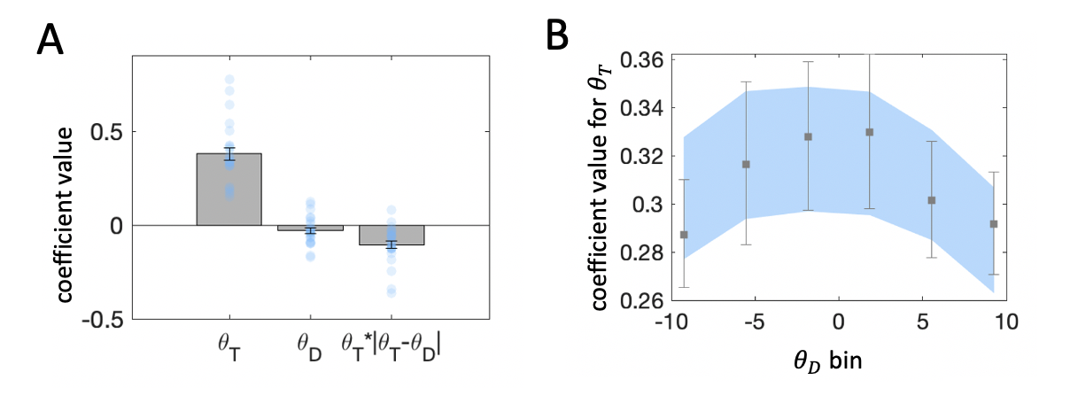
Figure 3.5: \(\textbf{A:}\) Beta coefficients from regression of choices on target and distractor orientation. Note that the interaction term is divided by 10, to ensure that unit changes in each predictor variable are reported in consistent terms. Grey bars denote averages, error bars denote standard error of the mean, blue dots represent individual participants. \(\textbf{B:}\) Beta coefficients for target orientation from binned regressions. Distractor orientation was divided in 6 equally spaced bins. Within each bin we estimated a binomial regression of choices on target orientation. Grey squares denote regression with human choice as the outcome variable, and error bars denote standard error of the mean. Blue region denotes standard error from the same regression, but with choice estimates derived from the regression model (from panel A) fit to human data.

The best-fitting coefficients \(\beta_1\), \(\beta_2\) and \(\beta_3\) are shown in Fig. 3.5a. Firstly, \(\theta_T\) holds significant sway over decisions (\(t_{23}=11.41\), \(p<0.001\)). This is expected because participants were instructed to discriminate the target item. Secondly, the effect of consistency, indexed by \(\beta_3\), was statistically significant at the group level (\(t_{23}=-5.09\), \(p<0.001\)). The negative sign of the coefficient means that the influence of the target on choices was greater when the target-distractor consistency was greater (i.e. a positive consistency bias).

Thirdly, the effect of \(\theta_D\) was more variable. It appears that the direction of influence of the distractor varied from individual to individual (\(\beta_2 = -0.03 \pm 0.075\)) and a \(t\) test conducted on \(\beta_2\) at the group level failed to reach significance at an \(\alpha\) level of \(.05\), (\(t_{23}=-1.99\), \(p=0.06\)). Although this coefficient was nonsignificant at the group level, the fits of the regression model to data from individual participants suggested that the inclusion of \(\theta_D\) was warranted by the variance it explained.

Fig. 3.5b illustrates the results of the binned regression analysis estimating the influence of the target on choices across different distractor values. Sensitivity to the target was reduced for more extreme distractor orientations, across both clockwise and counterclockwise orientations. This finding is expected from the consistency effect, because target and distractor are necessarily more different on average when one of them is at the extreme. This pattern of results is also captured by the predicted choices from the stepwise regression-identified model (Eq. (3.2)).

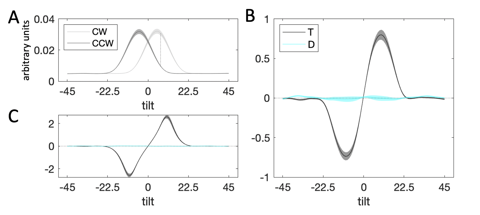
Figure 3.6: Decision kernel results. \(\textbf{A:}\) Average stimulus energy profiles. Dark grey curve denotes CCW stimuli, light grey curve – CW stimuli. Shaded regions correspond to M±SEM. The dashed line denotes maximum signal-to-noise ratio between the distribution for CW and CCW stimuli. \(\textbf{B:}\) Decision kernel based on participant choices. Black curve denotes the kernel for the target stimulus, cyan curve – the kernel for the distractor. Shaded regions correspond to M±SEM. \(\textbf{C:}\) Decision kernel based on ground truth stimulus tilts. Black curve denotes the kernel for the target stimulus, cyan curve – the kernel for the distractor. Shaded regions correspond to M±SEM.

3.2.2.2 Reverse Correlation

Fig. 3.6b illustrates the decision kernel for the target (black curve) and distractor (cyan line) stimuli averaged over all trials of the experiment. Positive kernel values indicate that an increase in energy at a given orientation is associated with higher probability of responding CW and negative kernel values – with responding CCW. The peak of the target kernel is on the CW side of orientation space, close to the maximum signal-to-noise ratio of the CW and CCW energy distributions (Fig. 3.6a, dashed line). Note that the kernel tapers towards zero beyond the range of -10° and 10° degrees from which stimulus orientations were sampled. A statistical test confirmed that while the average absolute value of the target kernel was significantly different from zero at orientations close to the decision boundary (i.e. \(|\theta|<22.5\)°, \(t_{23}=15.57\), \(p<0.001\)), it was not so at orientations far from the decision boundary (i.e. \(|\theta|>22.5\)°, \(t_{23}=1.78\), \(p=0.09\)). This pattern is also present in a decision kernel calculated based on the ground truth (whether the true stimulus orientation is CW/CCW) rather than participant responses (Fig. 3.6c, near the boundary: \(t_{23}=17.20\), \(p<0.001\), far from the boundary: \(t_{23}=0.99\), \(p=0.33\)).

In Fig. 3.6b, it can be seen that the decision kernel for the distractor was completely flat throughout orientation space. A statistical test on the average of the absolute values of the distractor kernel near the decision boundary (\(t_{23}=0.16\), \(p=0.87\)) and far from the boundary (\(t_{23}=-0.54\), \(p=0.59\)) confirmed that the kernel for the distractor did not deviate from zero. This is consistent with the fact that on its own, the angular offset of the distractor had an inconsistent impact on choices (\(\beta_2\) in the Eq. (3.2) regression).

To assess the interaction effect of the distractor, we next turn to the SVD results. The top 4 components derived from the target and distractor stimuli on each trial, which collectively accounted for 96% of the variance in filter energy (the first component captured 75% and the second – 16%), are shown in Fig. 3.7a. Of these 4 components, only component 2 had a different profile for the CW and CCW side of orientation space. Components 1, 3 and 4 were symmetric around the decision boundary. To confirm this intuition, we examined the component scores for each of the 4 components. A negative component score means that the variance in the stimulus is best captured by a mirror image of the component, flipped around the horizontal axis. In line with our visual inspection observations, on average, stimulus scores associated with components 1, 3 and 4 did not differ across CW and CCW oriented stimuli. By contrast, the stimulus scores for the second component appear to contain information pertaining to the tilt of the stimulus – they were predominantly positive for CW stimuli, and predominantly negative for CCW stimuli. Thus, we chose to use component 2 for our kernel regression analyses.

We regressed participant choices on the stimulus scores for the second component for the target \(U_T^2\) and distractor \(U_D^2\) on each trial, following the Eq. (3.2) regression model: \[\begin{equation} y = \beta_0 + \beta_1U_T^2 + \beta_2U_D^2 + \beta_3(U_T^2\cdot|U_T^2-U_D^2|) \tag{3.3} \end{equation}\]

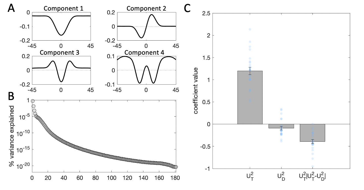
Figure 3.7: Kernel decomposition results. \(\textbf{A:}\) Illustration of the first four components yielded by singular value decomposition (SVD). \(\textbf{B:}\) Percentage of variance in the stimulus energy profile explained by each of the SVD components. Note that the y-axis is in logarithmic scale. \(\textbf{C:}\) Beta coefficients from a binomial regression of participant choices on stimulus scores for the second component and interactions with distractor signals. Grey bars denote averages, error bars denote standard error of the mean, blue dots represent individual participants.

Thus, the coefficient \(\beta_1\) reflects the independent effect of the target energy profile (as captured by component 2) on choices, \(\beta_2\) – the independent effect of the distractor profile, and \(\beta_3\) – the modulatory (interaction) effect of the distractor on sensitivity to the target, based on the consistency between target and distractor profiles. As expected, the main effect of the target profile on choices was strongly positive (\(t_{23}=14.67\), \(p<0.001\)). In this more sensitive analysis, however, distractor profiles now exerted a small direct repulsive effect on choices (\(t_{23}=-2.34\), \(p=0.03\)). Moreover, as expected from the analyses above, the distractor profile modulated the relationship between target profiles and choices (\(t_{23}=-8.80\), \(p<0.001\)), such that the more consistent the target and distractor profile, the stronger the relationship between target profile and choice.

3.2.3 Interim Discussion

Taken together, the results from both our classic and reverse correlation analyses suggest that the effect of distraction is primarily interactive, i.e. distractors modulate choices by virtue of the way they interact with targets. There may also be a more idiosyncratic independent effect of the distractor on choice. However, this effect was much weaker than the interactive effect and indeed nonsignificant on the group level in our classical regression analysis. The independent distractor effect identified in the reverse correlation analysis was repulsive, meaning that it pushed choices away from the orientation indicated by the distractor. We take these data to mean that the primary way in which distractors influences choices is interactive rather than independent.

3.3 Experiment 2

We next asked whether the interactive effect of distraction operates at the perceptual level or at the decision level. That is, is the contextual influence of the distractor driven by its sensory features or by its decision information? The interaction model has been proposed to operate across both sensory domains (e.g. in visual cortex, Kapadia et al. 1995) and in more abstract decision processes (e.g. about value-based information, Louie, Khaw, and Glimcher 2013). Our task features a low level visual property (orientation), suggesting that interactions between raw sensory information could be driving the effect. However, sensory level interactions have been documented at comparably closer locations in retinotopic space (U. Polat and Sagi 1994) relative to our task here, which positioned target and distractor in opposite visual hemifields. Thus, the effects we observe might instead be driven by interactions at later stages of processing of decision inputs.

To disentangle the perceptual and decision level information in our task, we orthogonalized the decision boundaries for target and distractor stimuli. Thus, in Experiment 2, target and distractor stimuli that share the same tilt relative to their respective boundary would be offset by 90° in terms of their raw tilts. We reasoned that if the contextual influence of the distractor occurred at the perceptual level and thus depended on similarity in terms of raw tilt, then the interaction effect would be null in Experiment 2 where this similarity is all but destroyed. Hence, any interaction effect that survives this manipulation must be due to encoding of information at the decision level (i.e. similarity of tilt relative to the boundary).

We analyzed the data from Experiment 2 in the frame of reference of the decision boundary. That is, we used stimulus tilt relative to the respective boundary rather than raw stimulus orientation in all our analyses. This allowed us to first, avoid wrap around effects in sensory similarity due to the circular nature of orientation space, and second, compare directly the magnitude of the decision level interaction effects between Experiments 1 and 2. If we see equivalent consistency effects in both experiments, this would indicate that the influence of the distractor occurs at the decision level.

3.3.1 Methods

3.3.1.1 Participants

Thirty-two participants (aged 24 ±4.75) took part in Experiment 2. Eight participants were excluded from the main analyses as the accuracy of their responses for one of the possible stimulus locations was at chance level (defined as in Experiment 1). The study received ethical approval from the Central University Research Ethics Committee at the University of Oxford (approval reference number: R51752/RE002). All participants provided written informed consent and were compensated £10 per hour for their time.

3.3.1.2 Apparatus

Participants were seated in a dark room approximately 60cm away from a computer monitor (60Hz refresh rate, 1080x1290 resolution, 23’ Dell LCD) with linearized output light intensities. As in Experiment 1, visual stimuli were created and presented with Psychophysics Toolbox Version 3 (PsychToolbox-3, Brainard 1997) for MATLAB.

3.3.1.3 Stimuli

Experimental stimuli were as in Experiment 1; the only difference was in stimulus orientation. In one of the two stimulus locations, the decision boundary was vertical like in Experiment 1. In the other location, the decision boundary was horizontal. In line with this, Gabor pattern orientation was drawn from a uniform distribution with range –10° to 10° offset from vertical or horizontal for the two respective stimulus locations. The average value of the contrast ratio for the noise in the stimuli produced by the staircase across participants was 0.42. This relatively higher signal contrast in Experiment 2 (versus 0.32 in Experiment 1) indicates that, on average, participants found the task harder when using two different decision boundaries. This is in line with the relatively higher number of participants excluded due to chance-level performance in this experiment (8 versus 2 in Experiment 1).

3.3.1.4 Experimental Procedure

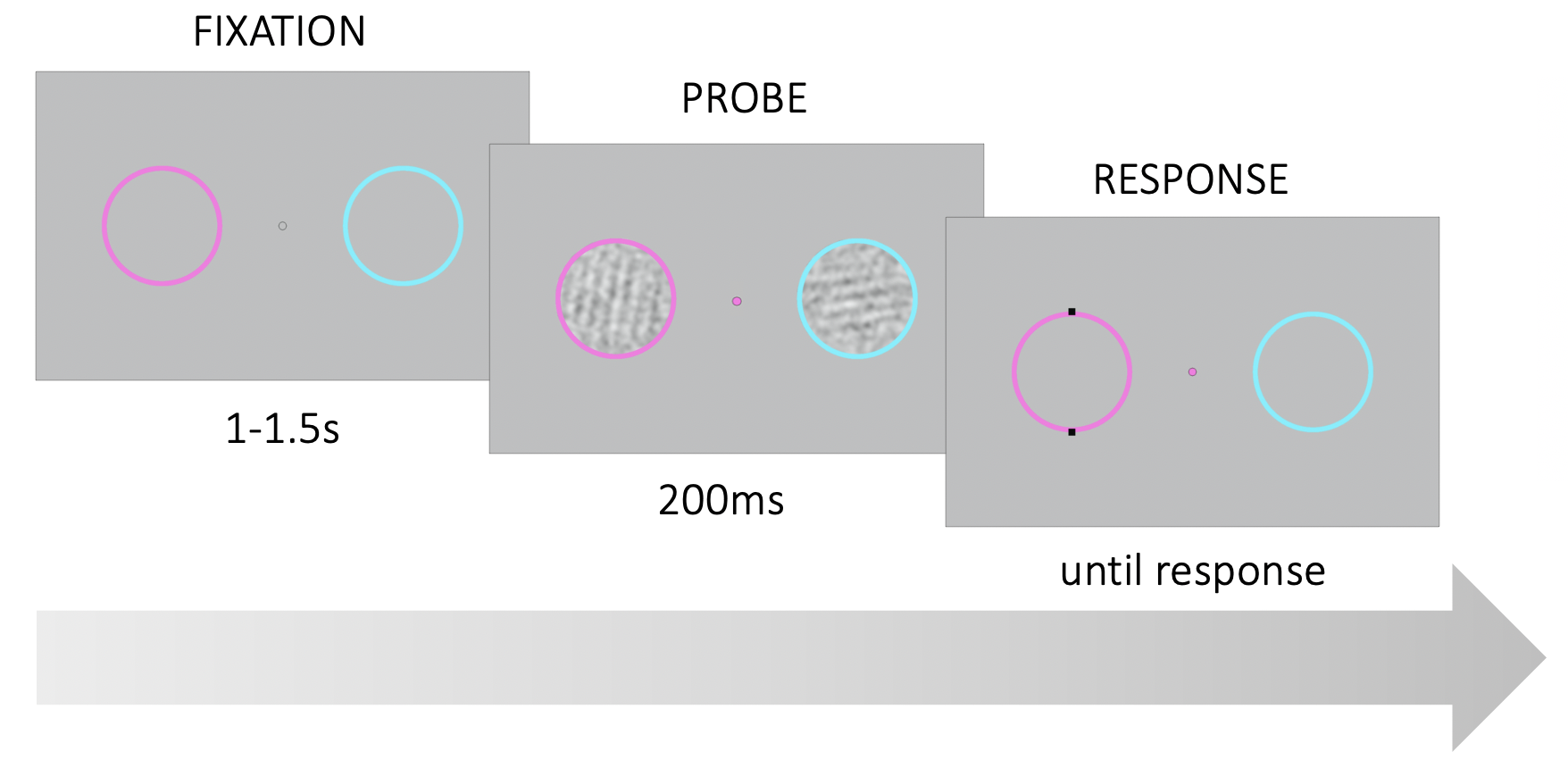
Figure 3.8: Trial structure followed Experiment 1. However, the two colored rings had different reference orientations. In the example here, the decision boundary for the pink ring was vertical, and horizontal for the cyan ring.

The experimental procedure followed that of Experiment 1 (Fig. 3.8). The only difference between the two experiments was in decision boundaries. In Experiment 2, for one of the colored rings the decision boundary was vertical, and for the other – horizontal. The decision boundaries were fixed for the duration of the experiment and ring-boundary combinations were counterbalanced between participants. Participants were reminded of the relevant decision boundary by two dots (oriented vertically or horizontally) overlayed over the target ring on each trial.

3.3.1.5 Analyses

We followed the same analysis plan as for Experiment 1. As stimulus features were coded as angular offset from the relevant decision boundary, all analyses were conducted in decision space rather than in the raw sensory orientation space.

3.3.1.6 Data & Code Availability Statement

All data and code to reproduce the analyses are available in the OSF repository (https://osf.io/54rf2/) for this project.

3.3.2 Results

3.3.2.1 Regression Results

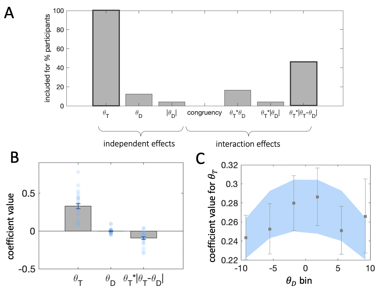
Figure 3.9: Regression results. Plots are as in Experiment 1. \(\textbf{A:}\) Results from stepwise regressions estimated individually for each participant in the experiment. Darker bar outlines indicate predictors we included in the final model. \(\textbf{B:}\) Beta coefficients from regression of choices on target and distractor orientation. \(\textbf{C:}\) Beta coefficients for target orientation from binned regressions.

Fig. 3.9a illustrates the results of the stepwise regression on participant choices. Interestingly, while the independent effect of the target and the interaction effect of distraction mirrored the findings from Experiment 1, the independent effect of the distractor explained a sufficient amount of variance to be included in the final model for only 3 out of 24 participants. Thus, the best fitting model for the choice data in Experiment 2 was: \[\begin{equation} y = \beta_0 + \beta_1\theta_T + \beta_3(\theta_T\cdot|\theta_T-\theta_D|) \tag{3.4} \end{equation}\]

As expected, the target had a strong positive influence on choices (\(t_{23}=9.89\), \(p<0.001\)) and the coefficient for the interaction effect of distraction was negative (\(t_{23}=-5.13\), \(p<0.001\)). For consistency with Experiment 1, we also report the results for the Eq. (3.2) model (Fig. 3.9b). The results for the target (\(t_{23}=9.40\), \(p<0.001\)) and the interaction effect of distraction (\(t_{23}=-5.43\), \(p<0.001\)) follow the same pattern. The coefficient for the independent effect of the distractor failed to reach statistical significance (\(t_{23}=-0.51\), \(p=0.62\)). Thus, in this experiment, the direction of the independent influence of the distractor again varied from individual to individual (\(\beta_2=-0.004 \pm 0.037\)), however, its inclusion in the model was not warranted by the amount of variance it explained in participant choices.

As can be seen from Fig. 3.9c, the results of the binned regression analysis followed closely those from Experiment 1. Across both participant and regression model-predicted choices, sensitivity to the target was reduced for more extreme distractor orientations, across both clockwise and counterclockwise orientations. This pattern of results is in line with the observed consistency bias.

3.3.2.2 Reverse Correlation

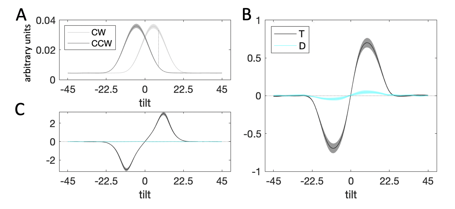
Figure 3.10: Decision kernel results. Plots are as in Experiment 1. \(\textbf{A:}\) Average stimulus energy profiles. \(\textbf{B:}\) Decision kernel based on participant choices. \(\textbf{C:}\) Decision kernel based on ground truth stimulus tilts.

Fig. 3.10b illustrates the decision kernel for the target and distractor. The target kernel follows the same pattern as in Experiment 1, with a peak on the CW side of feature space and a trough on the CCW side. Again, it tapered off to zero for angles away from the decision boundary (close to the boundary: \(t_{23}=13.06\), \(p<0.0001\), far from the boundary: \(t_{23}=1.27\), \(p=0.22\)). Interestingly, the distractor kernel appears slightly peaked in a way that follows the target kernel. Indeed, the average absolute value of the kernel at orientations close to the category boundary was significantly different from zero (\(t_{23}=2.47\), \(p=0.02\)), but further from the category boundary it was nonsignificant (\(t_{23}=0.17\), \(p=0.86\)). This suggests that participant choices were attracted, albeit rather weakly, towards the signal-like energy in the distractor.

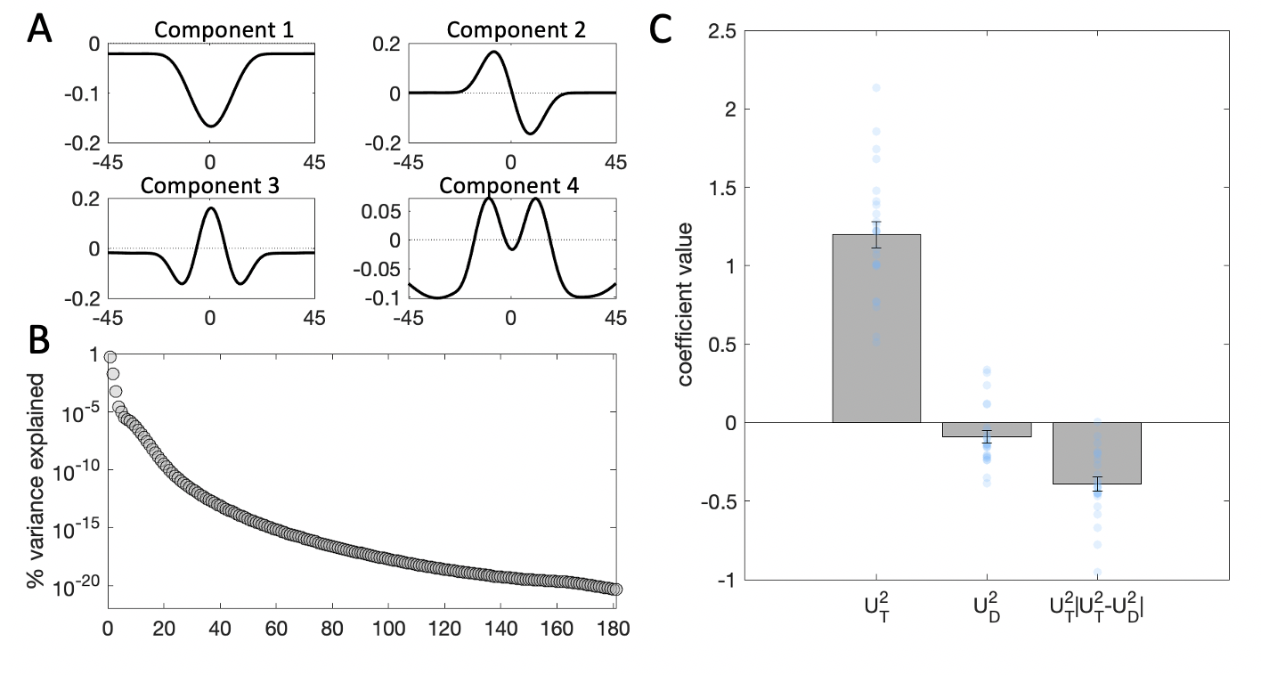
Figure 3.11: Kernel results. Plots are as in Experiment 1. \(\textbf{A:}\) Illustration of the first four components yielded by SVD. Note that the second component is a mirror image of the component resulting from Experiment 1. For ease of interpretability and consistency between the two experiments, we flipped the sign of the component scores for component 2 in the following analyses. \(\textbf{B:}\) Percentage of variance in the stimulus energy profile explained by each of the SVD components. \(\textbf{C:}\) Beta coefficients from a binomial regression of participant choices on stimulus scores for the second component and interactions with distractor signals. Grey bars denote averages, error bars denote standard error of the mean, blue dots represent individual participants.

The SVD regression analysis yielded analogous components as in Experiment 1 (Fig. 3.11a-b). This is perhaps unsurprising, as we followed the same stimulus generation procedure. The second component, however, was flipped compared to the second component derived from the stimuli in Experiment 1, suggesting that here, positive component scores would be associated with CCW stimuli, and negative component scores with CW stimuli. Thus, for ease of interpretability and consistency with Experiment 1, we multiplied \(U^2\) by \((-1)\) prior to fitting the Eq. (3.3) regression model (Fig. 3.11c). The results followed those from Experiment 1. We found a positive independent effect of the target (\(t_{23}=10.84\), \(p<0.001\)) and a negative interaction effect of target-distractor consistency (\(t_{23}=-7.94\), \(p<0.001\)). The independent effect of the distractor failed to reach statistical significance in this analysis, where, unlike in the simple \(t\) test above, we controlled for the interaction effect of the distractor (\(t_{23}=-1.19\), \(p=0.24\)).

3.3.3 Interim Discussion

Overall, the results of Experiment 2 replicate the main findings from Experiment 1. The effect of target-distractor consistency was similar across the two experiments despite the fact that here the decision boundaries for target and distractor were orthogonal (horizontal and vertical). This implies that the relevant features for target and distractor interact at the decision rather than at the perceptual level, i.e. at a stage in which they have been placed in a frame of reference that is relative to the decision boundary. The independent effect of the distractor was more elusive. Unlike Experiment 1, here the independent effect of the distractor was not included in the best fitting model. It also produced nonsignificant coefficients in regression analyses based on distractor tilt and distractor energy. Interestingly, while in Experiment 1 there were suggestions that the distractor may exert a weak repulsive influence on choices, here a small attraction effect was apparent in the distractor kernel.

Perhaps counter-intuitively, this pattern of results is actually in line with the direct repulsive influence of the distractor reported in Experiment 1 if the direct effect of the distractor occurs at the perceptual level. As analyses for Experiment 2 were carried out on the tilt offset of the two stimuli relative to two orthogonal boundaries, inputs that are close in decision space (e.g. tilt offsets 10° and 9° = 1° distance in decision space) are actually further in sensory space (respectively 10° and 99° = 89° distance in orientation space) compared to inputs that are more distanced in decision space (e.g. tilt offsets 10° and -9° = 19° distance in decision space, respectively 10° and 81° = 71° distance in orientation space). Thus, to interpret these results in the same frame of reference as the findings from Experiment 1, we should swap the sign of the effect. The relatively weaker direct effect here could be owing to the fact that target-distractor tilt pairs used in Experiment 2 were much more distant in orientation space compared to those in Experiment 1.

3.4 Experiment 3

Focusing attention on a decision-relevant location promotes target processing at the expense of distractors, and leads to heightened accuracy and faster reaction times (Posner, Snyder, and Davidson 1980; Hawkins et al. 1990; Carrasco 2011). This naturally raises the question of how the interactive effect of distraction described here changes when targets are, or are not, the focus of spatial attention. In Experiment 3, thus, we manipulated spatial attention by probabilistically cueing participants to focus on either the target or distractor stimulus in order to asses interactions with distraction.

3.4.1 Methods

3.4.1.1 Participants

Twenty participants (aged 24.3 ±3.69) took part in the Experiment 3. The study received ethical approval from the Central University Research Ethics Committee at the University of Oxford (approval reference number: R64927/RE001). All participants provided written informed consent and were compensated £10 per hour for their time.

3.4.1.2 Apparatus

Participants were seated in a dark room approximately 60cm away from a computer monitor (60Hz refresh rate, 1024x768 resolution, 17’ LCD) with linearized output light intensities. Visual stimuli were created and presented with Psychophysics Toolbox Version 3 (PsychToolbox-3, Brainard 1997) for MATLAB. Throughout the experiment, participants’ eye gaze position was monitored via eye-tracking using SR Research EyeLink 1000.

3.4.1.3 Stimuli

Experimental stimuli were generated as described in Experiment 1.

3.4.1.4 Experimental Procedure

Each participant completed the experiment in a single session, lasting approximately three hours. The experimental session consisted of 2 training mini-blocks of 50 trials each, an adaptive staircase and 9 test blocks of 200 trials each with a short break midway through each test block. The 2 training mini-blocks served to familiarize the participant with the task and the staircase followed the same procedure as in Experiments 1 and 2.

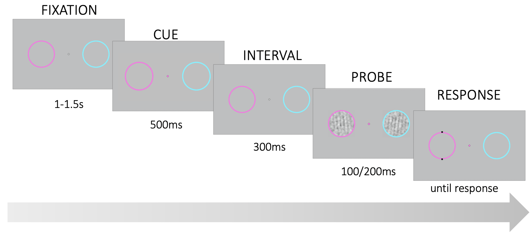
Figure 3.12: Trial structure followed Experiment 1. However, here, 800ms prior to stimulus presentation, the fixation point assumed the color of the ring which was more likely to be probed for 500ms. Note that on each trial stimulus duration was randomly determined as either 100ms or 200ms.

We adjusted the trial sequence in the test blocks to manipulate spatial attention via a spatial cue component (Fig. 3.12). The cue provided information about which stimulus was more likely to be the target. In 2 of the test blocks, the cue was neutral, and thus, trials were in practice equivalent to Experiment 1 (other than some small differences in trial timing). Participants were informed at the start of the neutral blocks that the cue would not be informative and the color of the fixation point (white) reflected this. In the remaining 7 blocks, the cue assumed the color of the ring which was more likely (70%) to be probed.

Each trial began with the probabilistic cue – the fixation point assumed the color of one of the two rings (or white in the neutral condition) for 500ms. 300ms following cue offset, two noisy gratings appeared within the colored rings for either 100ms or 200ms. Stimulus timings were randomized across trials to maximize the effect of cue validity on choice. At stimulus onset, the fixation point assumed the color of one of the two rings until the end of the trial. The color of the fixation point served as the probe indicating which of the two stimuli was the target. At stimulus offset, two dots were overlaid over the target ring. These dots corresponded to the vertical decision boundary relative to which participants had to report the tilt of the target. Participants reported their responses via keyboard presses (left and right arrow keys) and instantaneously received fully informative auditory feedback (correct: high tone, 880Hz and incorrect: low tone, 440Hz). Responses were not accepted on trials where the participant failed to maintain fixation, defined as gaze location further than 2° in radius from fixation. The experimenter remained in the same room as the participant to re-calibrate the eye tracker in between experimental blocks. Auditory feedback was delivered to the participant via headphones.

3.4.1.5 Analyses

We adapted the analytic strategy from Experiments 1 and 2, to assess the influence of spatial attention and its interaction with the effect of the distractor.

3.4.1.5.1 Manipulation checks

First, we conducted manipulation checks to confirm that our spatial attention manipulation was successful. We coded each trial in the experiment into three cueing conditions: 1) valid, where the probabilistic cue correctly signaled the target stimulus, 2) invalid, where the probabilistic cue incorrectly signaled the distractor stimulus, and 3) neutral, where the cue provided no information. We compared accuracy rates (converted to log odds to avoid violating the normality assumption) and response times (log transformed to again avoid violating the normality assumption) across these three cueing conditions via a GLM, controlling for the nonindependence of data points from the same observer. We followed up the results of the GLM with pairwise comparisons via \(t\) tests.

3.4.1.5.2 Regression Analyses

Collapsing across cueing condition, we followed the analytic pipeline from Experiments 1 and 2. To assess interactions with spatial attention, in addition to the predictors identified via the stepwise approach, we added cueing condition as an interaction term to each of the predictors. Valid, neutral and invalid cueing conditions were coded as 1, 0 and -1 respectively.

3.4.1.5.3 Reverse correlation

We repeated all reverse correlation analyses from Experiments 1 and 2, collapsing across cueing condition. To assess interactions with attention, we plotted kernels for each cueing condition separately. For the SVD regression analyses, we followed the same strategy as above – we included cueing condition as an interaction term to each of the predictors in the regression model.

3.4.1.6 Data & Code Availability Statement

All data and code to reproduce the analyses are available in the OSF repository (https://osf.io/54rf2/) for this project.

3.4.2 Results

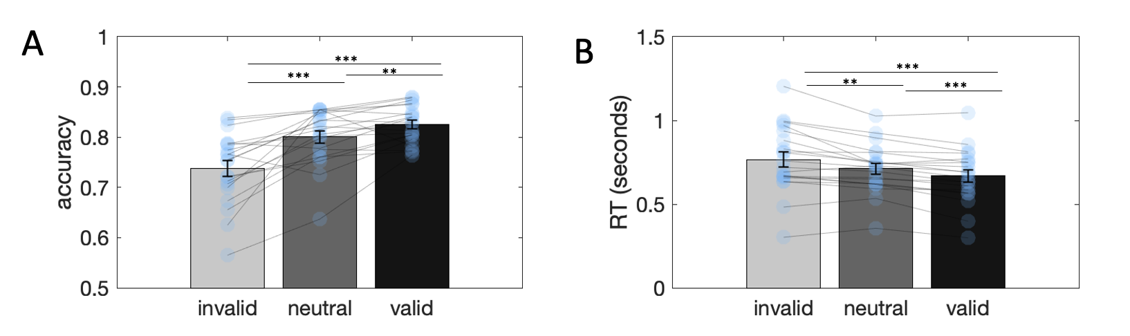
Figure 3.13: Attention manipulation check. \(\textbf{A:}\) Accuracy across invalid, neutral and valid trials. Statistical tests were performed on odds ratio transformed measures. \(\textbf{B:}\) Response times across invalid, neutral and valid trials. Statistical tests were performed on log transformed measures. Stars denote statistical significance: ** = p<0.01, *** = p<0.001.

3.4.2.1 Manipulation checks

Fig. 3.13 shows accuracy rates and response times across the three cueing conditions. As expected, accuracy was highest for valid trials and lowest for invalid trials, while response times followed the opposite pattern, indicating that our attention manipulation was successful. Log-transformed response time showed a valid < neutral < invalid pattern (GLM coefficient \(\beta=-0.07\), \(p<0.0001\); pairwise comparisons: valid < invalid: \(t_{19}=-8.76\), \(p<0.0001\), valid < neutral: \(t_{19}=-4.34\), \(p<0.0001\), neutral < invalid: \(t_{19}=-2.61\), \(p<0.02\)) and accuracy (transformed into log odds) showed a valid > neutral > invalid pattern (GLM coefficient \(\beta=0.26\), \(p<0.0001\); valid > invalid: \(t_{19}=6.07\), \(p<0.0001\), valid > neutral: \(t_{19}=3.00\), \(p<0.01\), neutral > invalid: \(t_{19}=4.82\), \(p<0.0001\)).

3.4.2.2 Regression Results

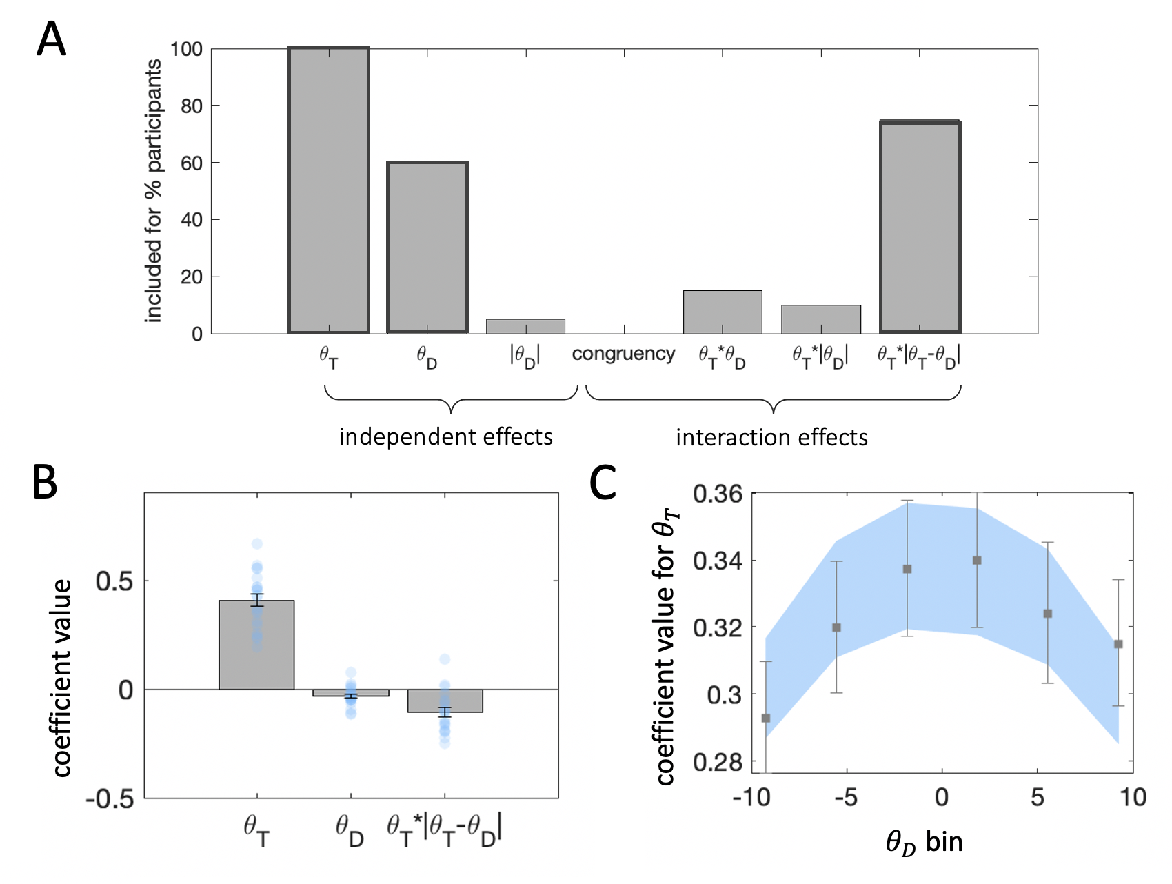
Figure 3.14: Regression results collapsing across cueing condition. Plots are as in Experiment 1. \(\textbf{A:}\) Results from stepwise regressions estimated individually for each participant in the experiment. Darker bar outlines indicate predictors we included in the final model. \(\textbf{B:}\) Beta coefficients from regression of choices on target and distractor orientation. \(\textbf{C:}\) Beta coefficients for target orientation from binned regressions.

First, we attempted to replicate the regression analyses from Experiments 1 and 2 collapsing across cueing condition. As can be seen from Fig. 3.14a, the stepwise regression identified the same predictors as in Experiment 1. Fitting Eq. (3.2) to the choice data from Experiment 3 replicated the strong sway of targets on choice (\(t_{19}=14.17\), \(p<0.001\)) and the target-distractor consistency effect (\(t_{19}=-5.00\), \(p<0.001\)). Here, the distractor had a statistically significant repulsive effect (\(t_{19}=-3.17\), \(p=0.005\)). The binned regressions produced the same pattern of results as in Experiments 1 and 2. Target sensitivity in participant and model-produced choices was reduced at more extreme distractor orientations, in line with the observed consistency bias.

Next, to assess the impact of target and distractor (and their interaction) under different attentional cueing conditions, we again used logistic regression (Fig. 3.17b), but now including interaction terms with attention (cueing) condition: \[\begin{equation} y = \beta_0 + \beta_1\theta_T + \beta_2\theta_D + \beta_3(\theta_T\cdot|\theta_T-\theta_D|) + \beta_4A\cdot\theta_T + \beta_5A\cdot\theta_D + \beta_6A\cdot(\theta_T\cdot|\theta_T-\theta_D|) \tag{3.5} \end{equation}\]

This expression looks a little complicated but in fact builds naturally from Eq. (3.2). The first three terms (associated with \(\beta_1\),\(\beta_2\) and \(\beta_3\)) are identical to those in Eq. (3.2). The final three terms are new predictors that encode the extent to which \(\theta_T\), \(\theta_D\) and their interaction influence choices as a function of cueing validity. In Eq. (3.5) thus \(A\) is an indicator variable coding cueing validity.

The results for \(\beta_{(1-3)}\) restate those described above (\(\beta_1\): \(t_{19}=13.57\), \(p<0.001\), \(\beta_2\): \(t_{19}=-2.68\), \(p=0.02\), \(\beta_3\): \(t_{19}=-4.69\), \(p<0.001\)). Attention modulated sensitivity to target orientations (\(\beta_4\): \(t_{19}=4.80\), \(p<0.001\)), as expected from previous work in the attention literature. Surprisingly, however, attention did not impact the direct effect of the distractor (\(\beta_5\): \(t_{19}=-1.46\), \(p=0.16\)), nor its modulatory influence on target sensitivity (\(\beta_6\): \(t_{19}=0.71\), \(p=0.49\)).

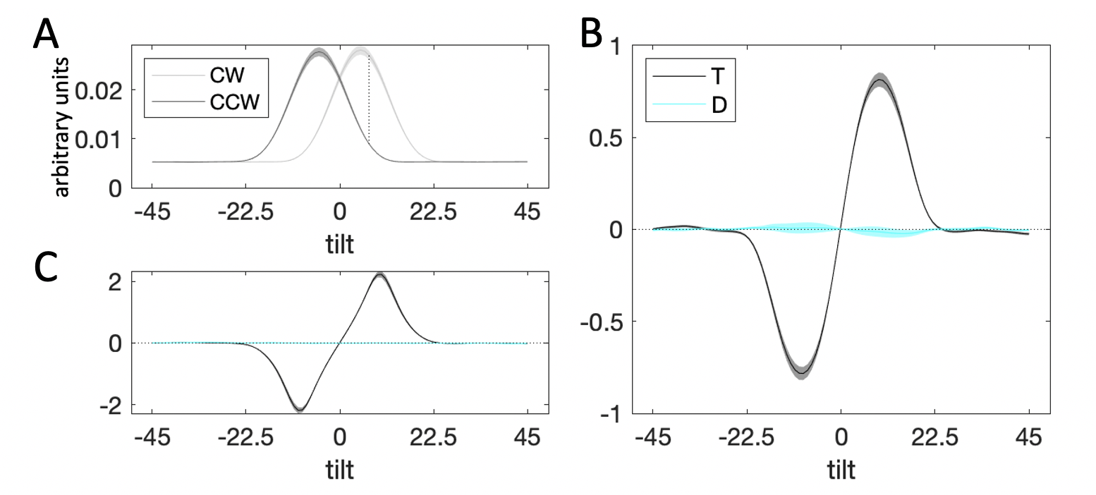
Figure 3.15: Decision kernel results collapsing across cueing condition. Plots are as in Experiment 1. \(\textbf{A:}\) Average stimulus energy profiles. \(\textbf{B:}\) Decision kernel based on participant choices. \(\textbf{C:}\) Decision kernel based on ground truth stimulus tilts.

3.4.2.3 Reverse Correlation Results

Again, we started by attempting to replicate the reverse correlation results from Experiments 1 and 2 collapsing across cueing condition. The kernel results were consistent with those above (Fig. 3.15). The target kernel significantly drove choices close to the category boundary (\(t_{19}=23.80\), \(p<0.001\)) and tapered off to zero for orientations further away from the boundary (\(t_{19}=-1.43\), \(p=0.17\)). The distractor kernel was flat throughout orientation space (near the category boundary: \(t_{19}=-0.55\), \(p=0.59\), far from the category boundary: \(t_{19}=0.09\), \(p=0.92\)).

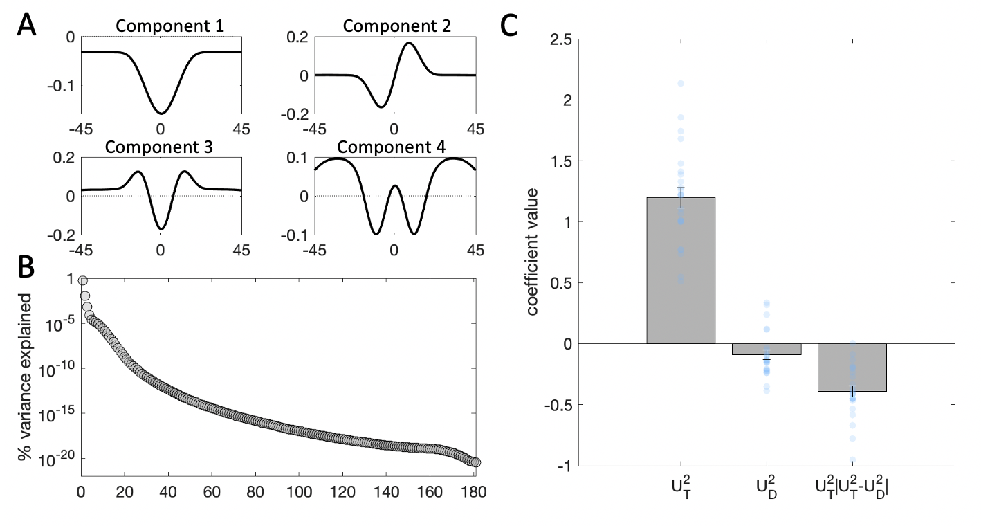
Figure 3.16: Kernel decomposition results collapsing across cueing condition. Plots are as in Experiment 1. \(\textbf{A:}\) Illustration of the first four components yielded by SVD. \(\textbf{B:}\) Percentage of variance in the stimulus energy profile explained by each of the SVD components. \(\textbf{C:}\) Beta coefficients from a binomial regression of participant choices on stimulus scores for the second component and interactions with distractor signals. Grey bars denote averages, error bars denote standard error of the mean, blue dots represent individual participants.

The SVD results (Fig. 3.16) and the regression based on component 2 replicated the findings from Experiment 1. The direct effect of the target profile on choices was strongly positive (\(t_{19}=18.72\), \(p<0.001\)) and we again observed the interaction effect of the consistency of target and distractor profiles on choice (\(t_{19}=-8.80\), \(p<0.001\)). Like in Experiment 1, we also observed a small direct repulsive effect of the distractor on choices (\(t_{19}=-3.29\), \(p=0.004\)).

Next, we considered these effects under different cueing conditions. Fig. 3.17a shows that there appears to be an attention-induced enhancement of target sensitivity in the decision kernels for the three different attention conditions. To quantitatively assess this, we re-ran the attention-inclusive regression model from Eq. (3.5) using the scores for component 2 as the predictor variables: \[\begin{equation} y = \beta_0 + \beta_1U_T^2 + \beta_2U_D^2 + \beta_3(U_T^2\cdot|U_T^2-U_D^2|) + \beta_4A\cdot U_T^2 + \beta_4A\cdot U_D^2 + \beta_6A\cdot(U_T^2\cdot|U_T^2-U_D^2|) \tag{3.6} \end{equation}\]

The results of this model replicated the results from the model based on angular offset \(\theta\) (Eq. (3.5)). The the target profile held a significant sway on decisions (\(\beta_1\): \(t_{19}=17.44\), \(p<0.001\)), the distractor profile exerted a repulsive influence (\(\beta_2\): \(t_{19}=-2.73\), \(p=0.01\)) as well as a negative interactive effect driven by its consistency with the target profile (\(\beta_3\): \(t_{19}=-9.63\), \(p<0.001\)). Crucially, cueing condition modulated sensitivity to the target (\(\beta_4\): \(t_{19}=5.12\), \(p<0.001\)), but had no impact on the direct effect of the distractor (\(\beta_5\): \(t_{19}=-1.66\), \(p=0.14\)), nor its modulatory influence on target sensitivity (\(\beta_6\): \(t_{19}=-1.15\), \(p=0.27\)).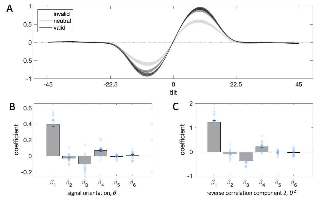

Figure 3.17: Results per cueing condition. \(\textbf{A:}\) Decision kernels for the target kernel in invalid, neutral and valid trials. Lightest grey denotes invalid, mid-grey – neutral and darkest grey – valid trials. \(\textbf{B:}\) Beta coefficients from a binomial regression on signal orientation. Grey bars denote averages, error bars denote standard error of the mean, blue circles denote individual participants. \(\beta_1\) is the coefficient for the target stimulus, \(\beta_2\) – the distractor, \(\beta_3\) – the interaction between target and the consistency between target and distractor, \(\beta_4\) – the interaction between target and cueing condition (coded as -1=invalid, 0=neutral, 1=valid), \(\beta_5\) – the interaction between the distractor and cueing condition, \(\beta_6\) – the three-way interaction between target, target-distractor consistency and cueing condition. \(\textbf{C:}\) As in B, but dependent variables in the regression correspond to the score for SVD component 2 from the reverse correlation analysis.

3.4.3 Interim Discussion

Collapsing across cueing condition, the results of Experiment 3 again replicate the interactive influence of the distractor. Here, we also observe a direct repulsive influence of distractors on choice, which we detected in only some of the analyses in Experiment 1. The observed contextual effects of irrelevant information do not differ across valid, invalid and neutral trials. This implies that directing attention heightens sensitivity to the imperative target stimulus, but, perhaps counter-intuitively, does not impact the contextual effects of irrelevant information.

3.5 Computational Modeling

The regression models above (Eq. (3.2)-(3.6)) were an analytic tool designed to partition variance in choice between independent predictors (\(\theta_T\) and \(\theta_D\)) and an interaction term \(f(\theta_T|\theta_D)\). However, there is a perhaps more elegant way to model the data, and one that, although closely related, makes more direct links to models of attention and contextual biasing that rely on normalization (Reynolds and Heeger 2009): \[\begin{equation} y = \frac{(x-\rho\cdot\mu)}{r+\tau\cdot\sigma} \end{equation}\]

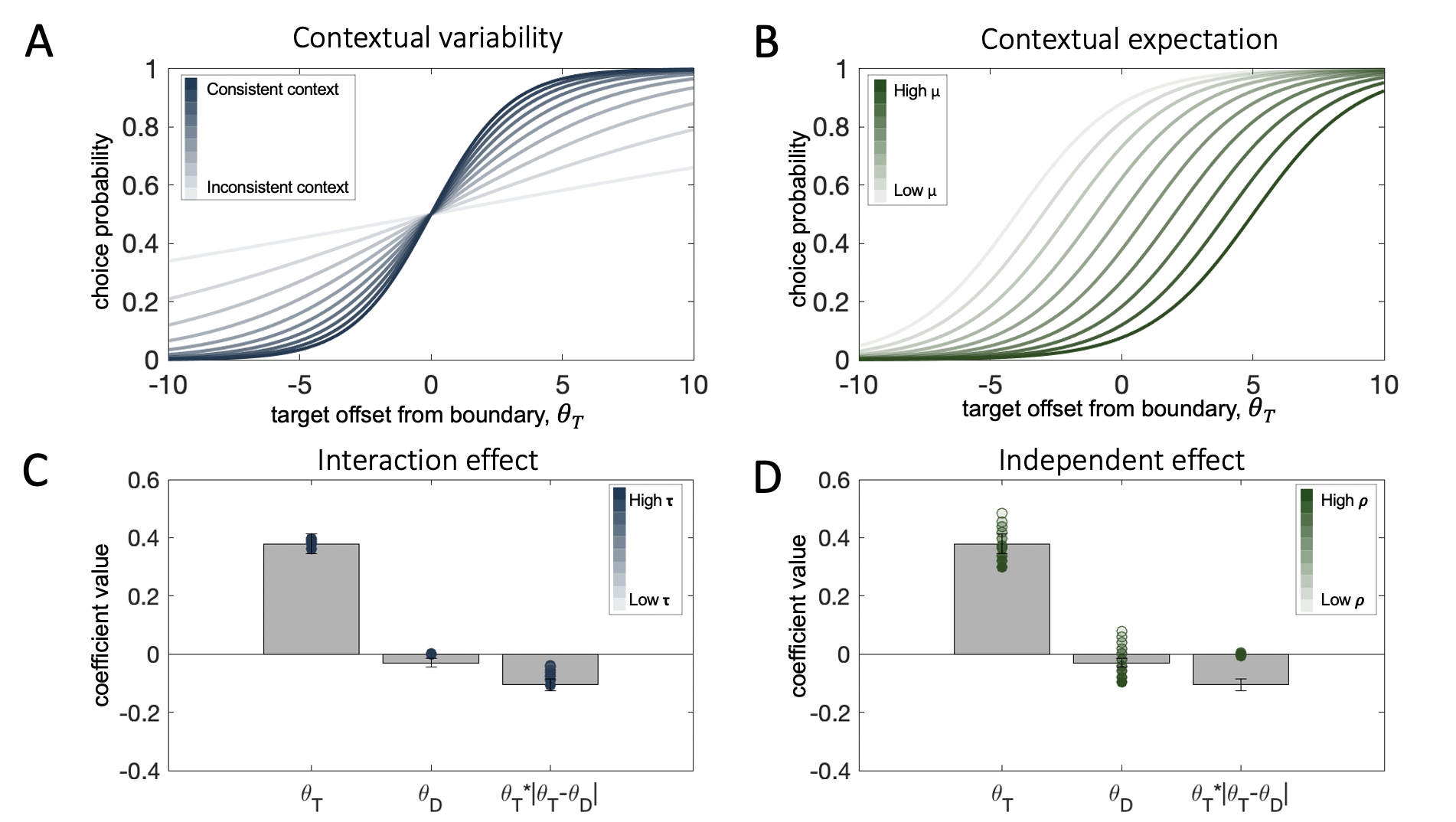
Figure 3.18: Model simulations of the effects of context on the transducer function translating decision inputs into choice probabilities (top) and on the distractor effects in choice behavior (bottom). \(\textbf{A:}\) The consistency of context changes the slope of the transducer. Lower contextual variability leads to steeper slope (darker blue curves) and vice versa for high variability (lighter blue curves). \(\textbf{B:}\) The contextual expectation changes the location of the inflection point of the transducer. A high contextual average leads to a transducer shifted rightwards along the x-axis (darker green curves) and vice versa for low contextual average. \(\textbf{C:}\) Contextual variability leads to an interaction effect of the distractor (target-distractor consistency). Bars correspond to coefficients from a regression on human choices from Experiment 1, filled circles correspond to an analogous regression on model simulations where we varied parametrically the value of \(\tau\), while keeping \(\rho\) and \(r\) constant. The higher the value of the multiplicative free parameter \(\tau\), the stronger the consistency effect (darker circles). \(\textbf{D:}\) The contextual expectation leads to an independent effect of the distractor. Bars correspond to coefficients from a regression on human choices from Experiment 1, filled circles correspond to an analogous regression on model simulations where we varied parametrically the value of \(\rho\), while keeping \(\tau\) and \(r\) constant. The higher the value of the multiplicative free parameter \(\rho\), the stronger the repulsion from the distractor (darker circles). Note that manipulations to \(\rho\) do not lead to an interaction effect (overlapping circles on last bar).

Here, \(y\) is the decision variable (as in Eq. (3.1)). A stimulus \(x\) is additively/subtractively modulated by the contextual biasing term \(\mu\) (in the attention literature this is sometimes known as a contrast gain effect, especially where the task involves detection) and multiplicatively/divisively normalized by a context variability term \(\sigma\) (similar to a multiplicative response gain effect). The degree of each type of gain control is respectively modulated by \(\rho\) and \(\tau\), and \(r\) is a regularizer; these 3 parameters are free to vary. Mapping this framework onto our experiment, the target feature \(x=\theta_T\), the context mean \(\mu=\frac{\theta_T+\theta_D}{2}\) and the context variability \(\sigma=|\theta_T-\theta_D|\), i.e. it is given by the range of the two targets. We chose this measure of contextual dispersion over the more commonly used standard deviation, as our experimental manipulation comprised only two stimuli (target and distractor).

This compact formulation of the model allows us to visualize how changes to context affect the (sigmoidal) transducer function linking decision inputs to choice (see Eq. (3.1)). Changes in contextual variability adjust the slope of the transducer – the more consistent the target and distractor, the steeper the slope (Fig. 3.18a), and consequently, the higher the gain of processing (Fig. 3.18c). The parameter \(\tau\) controls the degree of this change. As Fig. 3.18c shows, as \(\tau\) grows, the interaction effect of the distractor (target-distractor consistency) increases. By contrast, the contextual expectation shifts the transducer function along the abscissa (Fig. 3.18b). This impact translates into an independent effect of the distractor – for negative values of \(\rho\) we observe an attraction towards the distractor, and for positive values of \(\rho\) we observe a repulsion (Fig. 3.18d). This rich pattern of distractor influence maps onto the variability of the independent effect observed in human participants across the three experiments (the coefficient estimates for \(\beta_2\) in Eq. (3.2)).

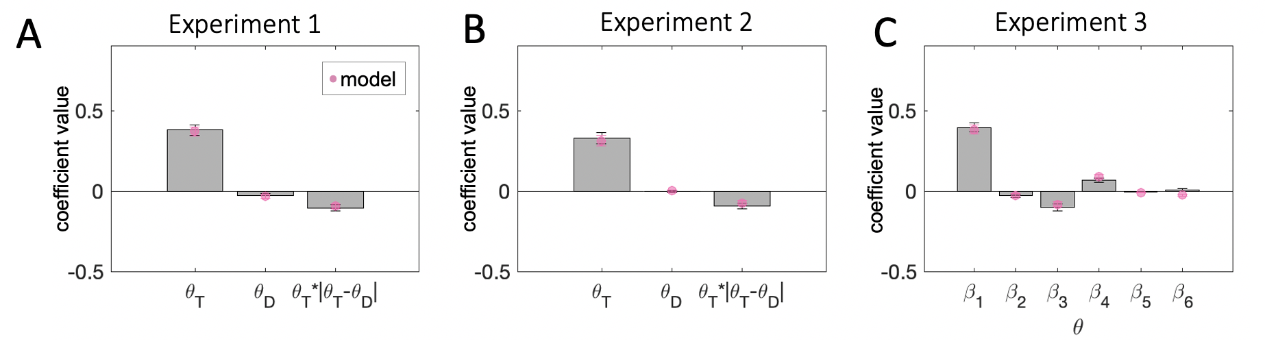
Figure 3.19: Model fits to human data. \(\textbf{A:}\) Experiment 1. \(\textbf{B:}\) Experiment 2. \(\textbf{C:}\) Experiment 3. Across all three experiments bars correspond to coefficients from a regression on human choices and pink circles correspond to model-simulated choices with free parameters estimated to best fit human data. Error bars correspond to standard errors of the mean. Coefficient labels in Experiment 3 are as in the regression analysis plot.

We fit this 3-parameter normalization model (\(r\), \(\tau\), and \(\rho\)) to human data from the first two experiments through gradient descent at the single trial level. Best fitting parameters were estimated for each participant individually by minimizing negative log likelihood. The model captures the pattern observed in the human data remarkably well (Fig. 3.19a-b). It recreates both the independent and interaction effect of the distractor. It is also quantitatively favored over a static model (where \(\tau=\rho=0\)) by Bayesian model selection on cross-validated model likelihoods (exceedance probabilities: Exp.1: \(p=0.99\), Exp.2: \(p=0.99\)).

To account for the observed effect of attention in Experiment 3, we allowed the parameter \(r\), which captures the baseline slope of the transducer above and beyond the impacts of contextual consistency, to vary freely across cueing conditions. Thus, in our process model, the spatial attention manipulation does not affect the strength of contextual normalization indexed by parameters \(\tau\) and \(\rho\). Rather, it changes the overall sensitivity to the target, as evidenced by the estimated parameter values: the slope of the transducer was steepest (i.e. lowest value for parameter \(r\)) in valid trials and shallowest (i.e. highest value for parameter \(r\)) in invalid trials (valid < invalid: \(t_{19}=3.94\), \(p<0.001\), valid < neutral: \(t_{19}=3.79\), \(p=0.001\), neutral < invalid: \(t_{19}=2.46\), \(p=0.02\)). Indeed, incorporating attention in this manner in the normalization model reproduced the observed changes in sensitivity to target orientation (Fig. 3.19c - \(\beta_4\)). Moreover, it captured the attention-independent effects of the distractor (\(\beta_2\) and \(\beta_3\)), as well as the lack of interaction of those with cueing condition (\(\beta_5\) and \(\beta_6\)).

3.6 Discussion

Across all three experiments, we found consistent evidence that distractors mainly influence choices by modulating the influence that targets have on choices. Our experiment involved a classic perceptual task – discrimination of noisy gratings – and our stimuli were spatially separated across the two hemifields, minimizing retinotopic visual interactions in the sensory encoding of target and distractor. Yet, our modelling suggests that targets have a stronger effect on choices when they are similar to distractors. This result was consistent using both conventional regression-based modeling and an approach based on reverse correlation analysis across all three experiments. This finding does not necessarily contradict, but does potentially nuance, previous accounts of distraction. For example, a standard model assumes that targets and distractors compete independently to influence choice, with the job of control processes being to upweigh targets at the expense of distractors.

In a different study, which is notable for applying a very rigorous modelling approach to a large body of data gathered from tasks that broadly resemble our own, the authors (Shen and Ma 2019) characterize the effect of distractor as being a generalized decrement to precision, or an increase in overall lapses of judgment (i.e. guess rate). However, their analysis does not attempt to ask how the features of target and distractor impact choices, but rather compares experimental conditions that have different levels of distraction, which might have led to their overlooking any interaction between target and distractor that is present in that data.

Relatedly, this finding is not consistent with a familiar framework for understanding decisions based on multiple, potentially noisy, sources of information with variable decision-relevance – that which is formalized by Bayesian inference (Dayan and Zemel 1999; Eckstein et al. 2009). In our experiment, a Bayesian ideal observer would weigh the target and distractor according to how relevant they were judged to be for the decision. How this relevance was determined would have to depend on some assumptions about the likely sources of error in the task, but in general, this class of explanation would point to decisions being determined exclusively by a weighted mixture of independent target and distractor features. This is not what we observed.

The form of the interactive effect we did observe seems related to a phenomenon has been previously described as a consistency bias (Cheadle et al. 2014). A consistency bias occurs when stimuli that resemble the local context are processed with heightened gain, and so have greater impact on choices. Previous work has reported a bias for decisions to be consistent with the recent temporal context, which is captured by a normalization model analogous to the one we discuss here (Cheadle et al. 2014). A closely related paper showed that a range of phenomena relating to spatial context – from across the subfields of perceptual, cognitive and economic decision-making – can be explained with a gain control model that also resembles the one described here (V. Li et al. 2018). Thus, seemingly unrelated phenomena such as the tilt illusion (Blakemore, Carpenter, and Georgeson 1970), congruency effects in a Flanker task (Eriksen and Eriksen 1974) and the distracting effect of decoy food items (Louie, Khaw, and Glimcher 2013) can all be captured by a closely related interactive model in which items that are similar to the context are processed with higher gain.

We observed an interaction between target and distractor decision values (tilt relative to the boundary) rather than perceptual values (raw tilt). This implies that the distractor, as well as the target, is placed in a frame of reference that expresses tilt relative to the category boundary. Consistent with this finding, a previous study using EEG found evidence from neural encoding that both target and distracting signals are placed in a decision-based frame of reference (Wyart, Myers, and Summerfield 2015), although of course it is likely that the extent to which selection occurs early or late depends on both the nature of the task and the available resources (Lavie and Tsal 1994). The data described here suggest that the interaction between target and distractor occurs at this later stage, beyond immediate sensory perception. This perhaps surprising result is in line with previous reports on the consistency bias (Cheadle et al. 2014) which also found that this effect occurred at a later stage of processing by dissociating sensory and decision inputs (via asking participants to make a decision based on the cardinality or diagonality of grating orientations). The finding that the contextual influence of perceptual distractors operates on decision level signals could perhaps also be anticipated from the many reports of contextual effects for stimuli that share an abstract property (such as value) but not a low level property (such as tilt), for example, in the literature on decoy effects discussed in the previous chapter.

We found limited evidence that the distractor impacted choices directly. The independent effect of the distractor appeared to largely vary idiosyncratically between participants both in terms of strength and direction. On the group level, this independent effect seemed to be reliable in Experiment 3, but was weaker in Experiment 1. Of note, these are the tasks for which the category boundary is the same for target and distractor, so it seems likely that any such effect (unlike the contextual consistency bias) operates at a perceptual, not a decision level. It is notable that the direction of the effect is repulsive, meaning that the more clockwise the distractor is, the less likely participants are to respond “clockwise.” The observed repulsion of choices from the sensory features of the distractor across Experiments 1 and 3 is also consistent with the weak independent effect we found in Experiment 2 (see section 3.2.3).

Indeed, contextual effects in sensory processing, such as adaptation over time (Webster 2015) and the tilt illusion (Blakemore, Carpenter, and Georgeson 1970), typically follow a repulsive pattern. The tilt illusion features grating stimuli similar to the ones we use here, however, the distracting flankers are closer to the target compared to in our set up. The higher degree of spatial separation can account for the weak and inconsistent nature of the sensory level effects we observe. Similar spatial interactions are documented in contrast perception (Chubb, Sperling, and Solomon 1989; Xing and Heeger 2001), where a central texture appears of lower contrast when surrounded by a high context texture compared to when surrounded by a uniform background. These psychophysical effects have previously been modeled in a normalization framework (Carandini and Heeger 2012). Here, we also demonstrate that the observed repulsive effect of the distractor can be captured by a model in which decision inputs are normalized by the contextual expectation. The direction of this effect cannot, however, be explained by a model in which target and distractor compete for attention and/or processing resources.

Finally, our findings also speak to the large literature which has explored the effect of attention on decisions made about a target stimulus in the face of distraction. In Experiment 3, we included a cueing manipulation that allowed us to test how attention might be deployed to mitigate the effect of distraction. Although we saw that spatial attention enhanced target processing – as demonstrated by both conventional and reverse correlation approaches – it did not seem to have any impact on the consistency bias. In other words, both target and distractor were elaborated into the frame of reference of the decision (Experiment 2) and then apparently interacted in a way that drove choices, but at no point (as far as we can see) did spatial attention intervene to facilitate or inhibit this process (Experiment 3). This finding seems hard to reconcile with physiological work with non-human primates, which shows that when spatial attention is directed towards a target stimulus, contextual modulation of neural responses by irrelevant stimuli in extra-striate area V4 is reduced by approximately 50% (Sundberg, Mitchell, and Reynolds 2009). This discrepancy might be related to the fact that the consistency bias appears to operate on the decision level rather than on the raw sensory signals likely captured by electrophysiological work in visual areas. In our data, spatial attention appeared to multiplicatively increase the gain with which a target stimulus is encoded (Carandini and Heeger 2012), but it did not modulate the independent or contextual effect of the distractor.

This pattern of results parallels findings on feature-based attention, which is known to operate broadly and independently of spatial attention (Liu, Stevens, and Carrasco 2007), and which has been associated with a feature-similarity gain control process not dissimilar from the consistency bias reported here. For example, when attention is cued towards a visual feature – such as downwards motion – in one part of the visual field, neurons sensitive to downwards visual motion (but with receptive fields at different locations) show heightened responses (Treue and Trujillo 1999). In attention studies, feature gain similarity also affects performance, albeit as potentially nonmonotonic function of target-distractor feature disparity (Störmer and Alvarez 2014; Liu 2019). However, in our study there was no overt cueing of features. One possibility is that there is an automatic feature-similarity gain process that depends on the context provided by the distractor. Future work can shed light on the relationship between the phenomena reported here, and the established literature on feature-based attention.

3.7 Conclusion

Perceptual decisions often occur in the presence of irrelevant information. Studies on attention have contributed greatly to our understanding of the behavioral signatures and neural underpinnings of focusing attention onto a target stimulus and away from irrelevant distractors. However, we know remarkably little about the influence distractors wield on choice. This chapter examined the functional relationship between the features of a distractor stimulus and perceptual decisions. Across three experiments, we found consistent evidence that distractors affect perceptual decisions primarily through an interactive effect, whereby consistency between target and distractor features boosts sensitivity to the target. This effect appears to operate on the level of the decision, rather than on raw sensory inputs, and is independent of attention. A simple normalization framework, where the dispersion of features present in the local context determines the gain of processing of decision-relevant information, can capture the behavioral signatures of distraction in our results, across all three experiments.

3.8 Acknowledgements

This chapter is submitted for publication and available as a preprint Dumbalska, T., Rudzka, K., Smithson, H. E., & Summerfield, C. (2021). How do (perceptual) distractors distract?.

Experiment 3 formed part of Katarzyna Rudzka’s final year undergraduate research project. Data collection for this experiment was carried out in its entirety by Katarzyna Rudzka. I am grateful for constructive feedback on an early draft of this chapter from my transfer of status assessors, Prof Jill O’Reilly and Dr MaryAnn Noonan. I also thank Prof Marisa Carrasco, members of her research group, and the participants in the Symposium on Biology of Decision Making (2019) for comments on presentations of this work.

References

Anderson, Britt. 2011. “There Is No Such Thing as Attention.” Frontiers in Psychology 2. https://doi.org/10.3389/fpsyg.2011.00246.

Ariely, Dan, George Loewenstein, and Drazen Prelec. 2003. “‘Coherent Arbitrariness’: Stable Demand Curves Without Stable Preferences.” QUARTERLY JOURNAL OF ECONOMICS, 33.

Barbot, Antoine, Valentin Wyart, and Marisa Carrasco. 2014. “Spatial and Feature-Based Attention Differentially Affect the Gain and Tuning of Orientation-Selective Filters.” Journal of Vision 14 (10): 703–3.

Blakemore, Colin, Roger H. S. Carpenter, and Mark A. Georgeson. 1970. “Lateral Inhibition Between Orientation Detectors in the Human Visual System.” Nature 228 (5266): 37–39. https://doi.org/10.1038/228037a0.

Brainard, David H. 1997. “The Psychophysics Toolbox.” Spatial Vision 10 (4): 433–36.

Bundesen, C. 1990. “A Theory of Visual Attention.” Psychol Rev 97 (4): 523–47.

Busemeyer, J. R., and J. T. Townsend. 1993. “Decision Field Theory: A Dynamic-Cognitive Approach to Decision Making in an Uncertain Environment.” Psychol Rev 100 (3): 432–59.

Carandini, M., and D. J. Heeger. 2012. “Normalization as a Canonical Neural Computation.” Nature Reviews Neuroscience 13 (1): 51–62. https://doi.org/10.1038/nrn3136.

Carrasco, M. 2011. “Visual Attention: The Past 25 Years.” Vision Res 51 (13): 1484–1525. https://doi.org/10.1016/j.visres.2011.04.012.

Cheadle, S., T. Egner, V. Wyart, C. Wu, and C. Summerfield. 2015. “Feature Expectation Heightens Visual Sensitivity During Fine Orientation Discrimination.” J Vis 15 (14): 14. https://doi.org/10.1167/15.14.14.

Cheadle, S., V. Wyart, Konstantinos Tsetsos, Nicholas Myers, Vincent de Gardelle, Santiago Herce Castañón, and Christopher Summerfield. 2014. “Adaptive Gain Control During Human Perceptual Choice.” Neuron 81 (6): 1429–41. https://doi.org/10.1016/j.neuron.2014.01.020.

Chelazzi, Leonardo, Francesco Marini, David Pascucci, and Massimo Turatto. 2019. “Getting Rid of Visual Distractors: The Why, When, How, and Where.” Current Opinion in Psychology 29 (October): 135–47. https://doi.org/10.1016/j.copsyc.2019.02.004.

Chubb, Charles, George Sperling, and Joshua A Solomon. 1989. “Texture Interactions Determine Perceived Contrast.” Proc. Natl. Acad. Sci. USA, 6.

Dayan, P., and R. Zemel. 1999. “Statistical Models and Sensory Attention.” In, 1017–22. London: International Conference on Artificial Neural Networks.

Desimone, Robert, and John Duncan. 1995. “Neural Mechanisms of Selective Visual Attention.” Annual Review of Neuroscience 18 (1): 193–222.

Eckstein, M. P., M. F. Peterson, B. T. Pham, and J. A. Droll. 2009. “Statistical Decision Theory to Relate Neurons to Behavior in the Study of Covert Visual Attention.” Vision Res 49 (10): 1097–1128. https://doi.org/10.1016/j.visres.2008.12.008.

Egner, T., and J. Hirsch. 2005. “Cognitive Control Mechanisms Resolve Conflict Through Cortical Amplification of Task-Relevant Information.” Nat Neurosci 8 (12): 1784–90. https://doi.org/10.1038/nn1594.

Eriksen, B. A., and C. W. Eriksen. 1974. “Effects of Noise Letters Upon the Identification of a Target Letter in a Nonsearch Task.” Perception & Psychophysics 16 (1): 143–49. https://doi.org/10.3758/BF03203267.

Geng, Joy J. 2014. “Attentional Mechanisms of Distractor Suppression.” Current Directions in Psychological Science 23 (2): 147–53. https://doi.org/10.1177/0963721414525780.

Gilbert, C. D., and W. Li. 2013. “Top-down Influences on Visual Processing.” Nat Rev Neurosci 14 (5): 350–63. https://doi.org/10.1038/nrn3476.

Hawkins, H. L., S. A. Hillyard, S. J. Luck, M. Mouloua, C. J. Downing, and D. P. Woodward. 1990. “Visual Attention Modulates Signal Detectability.” J Exp Psychol Hum Percept Perform 16 (4): 802–11.

Ito, Minami, and Charles Gilbert. 1999. “Attention Modulates Contextual Influences in the Primary Visual Cortex of Alert Monkeys.” Neuron 22 (3): 593–604. https://doi.org/10.1016/S0896-6273(00)80713-8.

Kapadia, Mitesh K., Minami Ito, Charles D. Gilbert, and Gerald Westheimer. 1995. “Improvement in Visual Sensitivity by Changes in Local Context: Parallel Studies in Human Observers and in V1 of Alert Monkeys.” Neuron 15 (4): 843–56. https://doi.org/10.1016/0896-6273(95)90175-2.

Krajbich, I., C. Armel, and A. Rangel. 2010. “Visual Fixations and the Computation and Comparison of Value in Simple Choice.” Nat Neurosci 13 (10): 1292–98. https://doi.org/10.1038/nn.2635.

Krause, Matthew R., and Christopher C. Pack. 2014. “Contextual Modulation and Stimulus Selectivity in Extrastriate Cortex.” Vision Research 104 (November): 36–46. https://doi.org/10.1016/j.visres.2014.10.006.

Landry, Peter, and Ryan Webb. 2021. “Pairwise Normalization: A Neuroeconomic Theory of Multi-Attribute Choice.” Journal of Economic Theory 193 (April): 105221. https://doi.org/10.1016/j.jet.2021.105221.

Lavie, Nilli, and Yehoshua Tsal. 1994. “Perceptual Load as a Major Determinant of the Locus of Selection in Visual Attention.” Perception & Psychophysics 56 (2): 183–97. https://doi.org/10.3758/BF03213897.

Li, Vickie, Elizabeth Michael, Jan Balaguer, Santiago Herce Castañón, and Christopher Summerfield. 2018. “Gain Control Explains the Effect of Distraction in Human Perceptual, Cognitive, and Economic Decision Making.” Proceedings of the National Academy of Sciences 115 (38): E8825–34. https://doi.org/10.1073/pnas.1805224115.

Liu, Taosheng. 2019. “Feature-Based Attention: Effects and Control.” Current Opinion in Psychology 29 (October): 187–92. https://doi.org/10.1016/j.copsyc.2019.03.013.

Liu, Taosheng, Sean T. Stevens, and Marisa Carrasco. 2007. “Comparing the Time Course and Efficacy of Spatial and Feature-Based Attention.” Vision Research 47 (1): 108–13. https://doi.org/10.1016/j.visres.2006.09.017.

Louie, K., M. W. Khaw, and P. W. Glimcher. 2013. “Normalization Is a General Neural Mechanism for Context-Dependent Decision Making.” Proceedings of the National Academy of Sciences 110 (15): 6139–44. https://doi.org/10.1073/pnas.1217854110.

Lu, Zhong-Lin, and Barbara Dosher. 2013. Visual Psychophysics: From Laboratory to Theory. MIT Press.

McAdams, C. J., and J. H. Maunsell. 1999. “Effects of Attention on Orientation-Tuning Functions of Single Neurons in Macaque Cortical Area V4.” J Neurosci 19 (1): 431–41.

Miller, E. K., and J. D. Cohen. 2001. “An Integrative Theory of Prefrontal Cortex Function.” Annu Rev Neurosci 24: 167–202. https://doi.org/10.1146/annurev.neuro.24.1.167.

Moran, J, and R Desimone. 1985. “Selective Attention Gates Visual Processing in the Extrastriate Cortex.” Science 229 (4715): 782–84. https://doi.org/10.1126/science.4023713.

Polat, U., and D. Sagi. 1994. “Spatial Interactions in Human Vision: From Near to Far via Experience-Dependent Cascades of Connections.” Proceedings of the National Academy of Sciences 91 (4): 1206–9. https://doi.org/10.1073/pnas.91.4.1206.

Posner, M. I., C. R. Snyder, and B. J. Davidson. 1980. “Attention and the Detection of Signals.” J Exp Psychol 109 (2): 160–74.

Reynolds, J. H., and L. Chelazzi. 2004. “Attentional Modulation of Visual Processing.” Annu Rev Neurosci 27: 611–47. https://doi.org/10.1146/annurev.neuro.26.041002.131039.

Reynolds, J. H., and D. J. Heeger. 2009. “The Normalization Model of Attention.” Neuron 61 (2): 168–85. https://doi.org/10.1016/j.neuron.2009.01.002.

Shen, Shan, and Wei Ji Ma. 2019. “Variable Precision in Visual Perception.” Psychological Review 126 (1): 89–132. https://doi.org/10.1037/rev0000128.

Soltani, Alireza, Benedetto De Martino, and Colin Camerer. 2012. “A Range-Normalization Model of Context-Dependent Choice: A New Model and Evidence.” Edited by Laurence T. Maloney. PLoS Computational Biology 8 (7): e1002607. https://doi.org/10.1371/journal.pcbi.1002607.

Stephan, Klaas Enno, Will D. Penny, Jean Daunizeau, Rosalyn J. Moran, and Karl J. Friston. 2009. “Bayesian Model Selection for Group Studies.” NeuroImage 46 (4): 1004–17. https://doi.org/10.1016/j.neuroimage.2009.03.025.

Störmer, Viola S., and George A. Alvarez. 2014. “Feature-Based Attention Elicits Surround Suppression in Feature Space.” Current Biology 24 (17): 1985–88. https://doi.org/10.1016/j.cub.2014.07.030.

Sundberg, Kristy A., Jude F. Mitchell, and John H. Reynolds. 2009. “Spatial Attention Modulates Center-Surround Interactions in Macaque Visual Area V4.” Neuron 61 (6): 952–63. https://doi.org/10.1016/j.neuron.2009.02.023.

Treue, Stefan, and Julio C. Martínez Trujillo. 1999. “Feature-Based Attention Influences Motion Processing Gain in Macaque Visual Cortex.” Nature 399 (6736): 575–79. https://doi.org/10.1038/21176.

———. 2015. “Visual Adaptation.” Annual Review of Vision Science 1 (1): 547–67. https://doi.org/10.1146/annurev-vision-082114-035509.

Wegener, Duane T., Richard E. Petty, Brian T. Detweiler-Bedell, and W.Blair G. Jarvis. 2001. “Implications of Attitude Change Theories for Numerical Anchoring: Anchor Plausibility and the Limits of Anchor Effectiveness.” Journal of Experimental Social Psychology 37 (1): 62–69. https://doi.org/10.1006/jesp.2000.1431.

Wyart, V., N. E. Myers, and C. Summerfield. 2015. “Neural Mechanisms of Human Perceptual Choice Under Focused and Divided Attention.” Journal of Neuroscience 35 (8): 3485–98. https://doi.org/10.1523/JNEUROSCI.3276-14.2015.

Wyart, V., A. C. Nobre, and C. Summerfield. 2012. “Dissociable Prior Influences of Signal Probability and Relevance on Visual Contrast Sensitivity.” Proc Natl Acad Sci U S A 109 (9): 3593–98. https://doi.org/10.1073/pnas.1120118109.

Xing, J., and D. J. Heeger. 2001. “Measurement and Modeling of Center-Surround Suppression and Enhancement.” Vision Research 41 (5): 571–83. https://doi.org/10.1016/S0042-6989(00)00270-4.