2 A map of decoy influence in multialternative economic choice
When choosing between two alternatives, the addition of a third inferior option should not affect choices. In practice, however, even though the dispreferred decoy good is rarely chosen, it can systematically sway preference towards one of the two original alternatives. Previous work has identified three classic decoy biases, known as the attraction, similarity and compromise effects, which arise during choices between economic alternatives defined by two attributes. However, the reliability, interrelationship, and computational origin of these three biases has been controversial. Here, a large cohort of human participants made incentive-compatible choices among assets that varied in price and quality. Instead of focusing on the three classic effects, we sampled decoy stimuli exhaustively across bidimensional multiattribute space and constructed a full map of decoy influence on choices between two otherwise preferred target items. Our analysis revealed that the decoy influence map was highly structured even beyond the three classic biases. We identified a very simple model that can fully reproduce the decoy influence map and capture its variability in individual participants. This model reveals that the three decoy effects are not distinct phenomena but are all special cases of a more general principle, by which attribute values are repulsed away from the context provided by rival options. The model helps understand why the biases are typically correlated across participants and allows us to validate a new prediction about their interrelationship. This work helps clarify the origin of three of the most widely studied biases in human decision-making.
2.1 Introduction
Optimal decisions should be driven solely by information that is relevant for the choice. When deliberating among more than two options (“multialternative” choices) this means ignoring those alternatives that are inferior or unavailable. Hence, the choice between two consumer goods should not be affected when an unaffordable third option is introduced. Similarly, voting preferences between two electoral candidates should not be changed when a third contender with more dubious merit enters the race. This normative principle, which is enshrined in the axiom of regularity (Block and Marschak 1960; Rieskamp, Busemeyer, and Mellers 2006), has been of significant and long-standing interest to behavioral scientists as it is robustly violated by a variety of animals including humans (A. Tversky 1972; J. Huber, Payne, and Puto 1982; Simonson 1989), monkeys (Parrish, Evans, and Beran 2015), amphibians (Lea and Ryan 2015), invertebrates (Shafir 1994), and even unicellular organisms (Latty and Beekman 2011). The existing empirical evidence has indicated that where choice alternatives are characterized by two value dimensions (e.g. the price and the quality of a product or the likability and competence of a political candidate), the introduction of an irrelevant distractor item to the choice set leads to rich and stereotyped biases in decision-making. A key research goal in the fields of psychology and economics has been to identify a simple and elegant computational principle that can explain the biases provoked by an irrelevant “decoy” stimulus (Turner et al. 2018).
The existing literature has focused on three decoy effects that can arise during ternary (three-way) choice among alternatives characterized by two independent and equally weighed attributes. The phenomena are illustrated in Fig. 2.1. Consider for example a consumer who is choosing between three products that are each characterized by dimensions (attributes) of quality and economy. The axes in Fig. 2.1 are scaled such that these attributes are perfect substitutions in that the consumer will forego one unit of one attribute for one unit of the other. Two target items, A and B, lie on the line of isopreference which is perpendicular to the identity line. In other words, A is less expensive but lower quality than B, such that the consumer should be indifferent between these options. The empirical phenomena describe how preferences may be biased towards either A or B as a function of a third “decoy” item D that lies on or below the isopreference line. The consensus view holds that a bias towards A can be provoked by the inclusion of a decoy \(D_a\) that it dominates, that is where A (but not B) is equivalent or superior on both dimensions (the attraction effect); that a bias towards A occurs in the presence of a more extreme decoy \(D_c\) which is superior in quality but yet more expensive than A, making A the “compromise” option (the compromise effect); and that a bias towards A is incurred by a decoy \(D_s\) which is similar to B in price and quality (the similarity effect, Fig. 2.1).
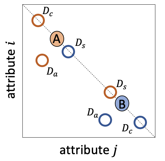
Figure 2.1: Illustration of the attraction, compromise and similarity effects. A and B denote two equally preferred stimuli; A is strong on attribute \(i\) but weak on attribute \(j\) and vice versa. The introduction of decoy stimuli (rings; denoted \(D_a\), \(D_c\) and \(D_s\)) can bias preferences towards either A or B. The color of each ring signals the direction of the bias, e.g. for orange rings, A is preferred. Stimuli falling on the dashed line are equally preferred.
These three phenomena have been a major object of study in psychology and behavioral economics for several decades, with research interest reinvigorated in the last couple of decades after a landmark study that proposed the first unified computational account of the three classic decoy effects (Roe, Busemeyer, and Townsend 2001). Since then, a variety of empirical results have been produced and a plethora of computational models have emerged. These include models that rely on loss aversion (K. Tsetsos, Usher, and Chater 2010), pairwise normalization (Landry and Webb 2021), attentional weighing (Hotaling, Busemeyer, and Li 2010; Konstantinos Tsetsos, Chater, and Usher 2012; Bhatia 2013; Trueblood, Brown, and Heathcote 2014), lateral inhibition (Hotaling, Busemeyer, and Li 2010), associative biases (Bhatia 2013), power-law transformation of attribute values (Bhatia 2013), sampling from memory (Noguchi and Stewart 2014; Bhui and Gershman 2018), or various other forms of reference-dependent computation (Soltani, De Martino, and Camerer 2012; V. Li et al. 2018; Natenzon 2019; Rigoli 2019). However, there has been a notable lack of consensus about the computational principles that give rise to decoy effects (Turner et al. 2018). There are a number of potential reasons for this, but here we focus on one limitation of past studies: most have tested for decoy effects by selecting fixed attribute values for \(D_a\), \(D_c\) and \(D_s\) and calculating for each the relative choice share (RCS) for target items A and B, with relative deviations from choice equilibrium signalling a bias indicative of the successful detection of a decoy effect. However, reducing the dimensionality of the data in this way (i.e. to 6 data points) makes it harder to distinguish theoretical accounts, as many models may mimic one another in successfully capturing the phenomena, so that comparisons among models are reduced to questions of a priori plausibility and parsimony. Relatedly, what defines a “decoy” of each class is typically left largely to the discretion of the researcher, who is free to choose a priori the values for \(D_a\), \(D_c\) and \(D_s\) – i.e. the space over which the attraction, compromise or similarity might occur. This issue, coupled with the fact that the effects are often studied in small participant cohorts, using diverse stimulus materials – consumer choices (Josiam and Hobson 1995), text-based vignettes (Yang and Lynn 2014), or perceptual judgments (Trueblood et al. 2013) – has led to disagreement over the provenance and reliability of the three effects (Trueblood 2012; Frederick, Lee, and Baskin 2014; Yang and Lynn 2014; Trueblood, Brown, and Heathcote 2015).
In this chapter, we address these issues by reporting a large-scale (\(n>200\)), incentive-compatible study. We systematically mapped the decoy influence across attribute space, calculating the relative choice share \(RCS_{ij}\) for each decoy with attribute values \(i\) and \(j\). This allowed us to explore the dimensionality of the data, with a view to asking whether a single principle can explain the ensemble of observed decoy effects. We found that a remarkably simple model, which draws on a computational framework based on the principle of divisive normalization, can capture the full decoy influence (RCS) map. Importantly, the model suggests that the three canonical decoy effects are not in fact distinct phenomena but rather fall naturally out of previously described dynamics of attraction and repulsion of decision values towards and away from a reference value given by the mean of available options.
2.2 Experiment
2.2.1 Methods
2.2.1.1 Participants
A total of 358 US-based participants were recruited via the platform Amazon Mechanical Turk to participate in a three-phase online study. All participants took part in the first phase (rating task), and those who passed a performance threshold (\(n=231\); see below) were invited to join the second and third parts of the study in separate testing sessions (choice task). Of these, 189 met our criteria for inclusion in the analysis, namely \(p<0.001\) of responding randomly during the choice task (binomial test). Phases 2 and 3 (choice task) were identical; phase 3 simply allowed us to gather more data (\(n=149\) completed both phases 2 and 3). Data were collected in two distinct batches. In the first batch, we paid participants $4 for completing each phase, in addition to a performance-based bonus of up to $20 for the second and third part of the study (a maximum payment of $32). To reduce the dropout rate, in the second batch the base payment was increased to $5 and the bonuses increased to $12 and $18 in the second and third phases respectively (a maximum payment of $45). The study received ethical approval from the Central University Research Ethics Committee at the University of Oxford (approval reference number: R50750/RE001).
2.2.1.2 Experimental Tasks
2.2.1.2.1 Rating Task
The first phase of the study (rating task, Fig. 2.2a) was introduced as a “property rental price guessing game.” The task involved estimating the market rental price of residential real estate by viewing an image of the exterior of a series of properties. On each trial, an image of a property was shown along with a horizontal slider for a maximum of 60 seconds. The task was to guess the market rental price of the property, i.e. the dollar amount that an average person would be willing to pay per month to rent it, and to indicate it on a slider scale. The slider ranged from $0 to $2500 and the initial position of the slider was randomized on each trial. There were a total of 250 unique house images, each presented twice in randomized order (for a total of 500 trials per participant). The 250 houses had been selected to have the lowest average choice variability in a pilot study involving 30 distinct participants and a larger set of properties (\(n=450\)), which we conducted before the main experiment. We used participant ratings from the pilot dataset to include/exclude participants. After phase 1, we correlated the 250 ratings for each participant against the average ratings obtained from the pilot study. Participants with a Spearman’s rank correlation of \(\rho< 0.7\) were excluded; the rest (\(n\) = 231) were invited to progress to the choice task.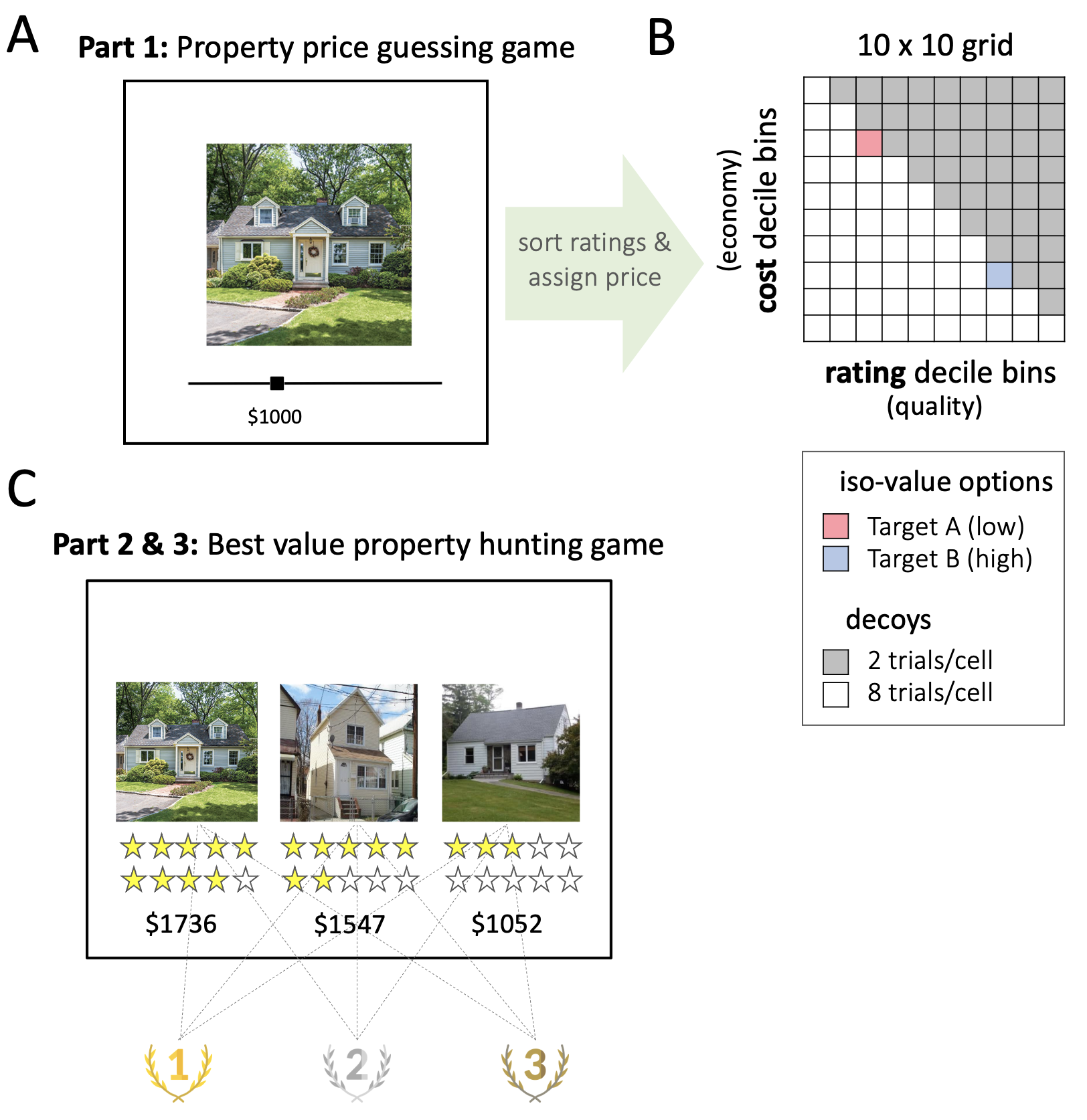
Figure 2.2: Experimental design. \(\textbf{A:}\) Participants first played a “property price guessing game.” On each trial they estimated the monthly rental value (in dollars) of a residential property, using a sliding scale. \(\textbf{B:}\) After discarding properties with inconsistent responses, ratings were sorted into deciles for each participant. These bins were used to select stimuli for targets A and B (deciles 3 and 8 of estimated ratings; red and blue squares), and decoy stimuli. Each choice task stimulus was created by matching a property with a given decile estimated value (quality; attribute \(j\)) to a new rental price (economy; attribute \(i\)) on a 10x10 grid. Eight property/price combinations were generated for each cell in the grid that lay below the diagonal (white cells), and 2 property/price combinations for each cell above the diagonal (grey cells). \(\textbf{C:}\) Participants then played a “best value property hunting game” in which they were asked to rank 3 stimuli according to their economy/quality trade off. Two of the stimuli corresponded to the targets A and B, the third stimulus was the decoy. A star rating system was used as a reminder of their previous price estimation judgment.
2.2.1.2.2 Choice Task
We introduced phases 2 and 3 as a “best-value property hunting game” (choice task, Fig. 2.2c). Here, participants were told to imagine that they were a real estate agent recommending to a client the best value house we, a fictitious real estate company, have on offer. On each trial, 3 properties (i.e. choice alternatives) were displayed for a maximum of 60 seconds on left, central and right positions on the screen. Underneath each image we displayed an allocated rental cost (in dollars) and a number of stars. The number of stars was proportional to the value given by the participant in the ratings task, and merely served as a reminder. In piloting, we found that this improved choice consistency. Participants were informed that the property images were a subset of those that they had viewed in phase 1, and that that the stars were related to the ratings they themselves had reported. The task asked participants to press three keyboard buttons (left, down, and right arrow buttons) to indicate their ordered preference from the best-valued house to the worst-valued house. Participants were explicitly instructed that the best-valued house was the one with the highest market value but the lowest allocated rental price. At the end of each block, participants were told how many trials’ recommendations were correct, given their initial ratings. The bonus payment at the end of each phase was proportional to their accuracy.
Unbeknownst to participants, the options were carefully selected for each participant individually to allow us to test our hypotheses of interest (Fig. 2.2b). First, for each participant we filtered out the 90 properties with the highest rating variability, i.e. the highest absolute deviance between the two ratings. Second, the remaining 160 properties were binned into quality deciles (attribute \(i\)) on the basis of each participant’s ratings. The binned properties could then be associated with an allocated rental cost that was drawn uniformly from within the range of dollar values that defined each decile (attribute \(j\)). This allowed us to select, on each trial, three stimuli that differed on two dimensions: two targets A and B, and a decoy stimulus. Target A was always a property drawn from the 3rd decile of quality (i.e. participant rating) and the 8th decile of economy (i.e. the 3rd decile of cost); target B was always drawn from the 8th decile of quality and the 3rd decile of economy (i.e. the 8th decile of cost). The decoy stimulus was sampled exhaustively from the full attribute space (any of the 10 quality x 10 economy bins). Thus, targets A and B were equally valued options (A being low quality and low cost, and B being high quality and high cost) and the decoy stimulus could be both superior or inferior in value. Participants completed a total of 530 trials in the second part of the study. The third part constituted an additional 530 trials of the same task.
2.2.1.3 Analyses
We calculated relative choice share for the “low” item A over the “high” item B by calculating the proportion of trials for which A was chosen before B across all trials in each decoy decile bin. We were able to do this for both inferior and superior decoys, as participants provided us with ranked preference for all three items. Thus, even if on a given trial they chose the decoy, they still reported whether they preferred A over B or vice-versa. This allowed us to plot the relative preference for A over B across the full attribute space (\(RCS_{ij}\)).
2.2.1.3.1 Conventional Decoy Analyses
We first adopted a standard approach from previous studies that have focused on estimating the effects of the three classic decoy effects, that is, calculating RCS for \(D_a\), \(D_c\) and \(D_s\). To this end, we defined portions of the influence map that corresponded to the traditionally defined positions of attraction, compromise and similarity decoys (Fig. 2.3a). We also included an additional decoy set that we called “repulsion” decoys (\(D_r\)): these were mirror-symmetric to the attraction decoys but located in the upper triangle of the influence map where the decoy was the objectively best option (i.e. a set of “superior” decoys). We then calculated the RCS for \(D_a\), \(D_c\), \(D_s\) and \(D_r\), each defined with respect to target A and target B. The strength of each effect was defined as the difference in RCS for each decoy set defined with respect to targets A and B. We tested each effect against zero for statistical significance via a single sample \(t\) test.
2.2.1.3.2 Interrelationship of Effects
To investigate the associations between the three classic decoy effects in our cohort, we calculated Pearson’s correlation coefficients. We estimated those pairwise for each of the three possible combinations of effects (\(D_c\)-\(D_a\), \(D_c\)-\(D_s\), and \(D_a\)-\(D_s\)), based on the strength of the effects for each participant in our sample.
2.2.1.3.3 Map of Decoy Influence
Our major goal for this project was to go beyond conventional analyses and chart decoy influence across the attribute space. The ordered RCS for option A over B in each decoy decile bin across all possible attribute combinations constitutes the map of decoy influence. In addition to the decoy map, as a sanity check, we also plotted preferences for the two targets over the decoy item. We did this by calculating the RCS for option A over the decoy D (i.e. in what proportion of trials did the participant choose A before D?), as well as the RCS for option B over the decoy D in each of the 10x10 decoy decile bins.
2.2.1.3.4 Map Decomposition
The resulting map of decoy influence allowed us to not only ask how the three classic decoy effects are interrelated in our cohort of participants, but to seek structure beyond these three locations in attribute space. Using an exhaustive range of decoy locations allowed us to use dimensionality reduction approaches to examine the (potentially distinct) factors from which the map of decoy influence is composed. We used singular value decomposition (SVD) to identify factors contributing to the map of preference for A > B and calculate the variance explained by these factors. To this end, we flattened the 10x10 decoy map for each participant into a vector of values and constructed a large matrix of RCS, where each row indexed an individual participant and each column – the decoy location in attribute space. SVD produces a set of basis functions, or factors, and allows us to examine the amount of variance explained by them in the empirical data. This, in turn, illustrates the structure of decoy effects across participants. Knowing this structure can give us clues as to whether distinct mechanisms drive decoy influence across different locations in attribute space, or alternatively, if the general structure of RCS can be explained by a single factor.
2.2.1.4 Data & Code Availability Statement
All data and code to reproduce the analyses are available in the OSF repository (https://osf.io/u6br3/) for this project.
2.2.2 Results
2.2.2.1 Conventional Decoy Analyses
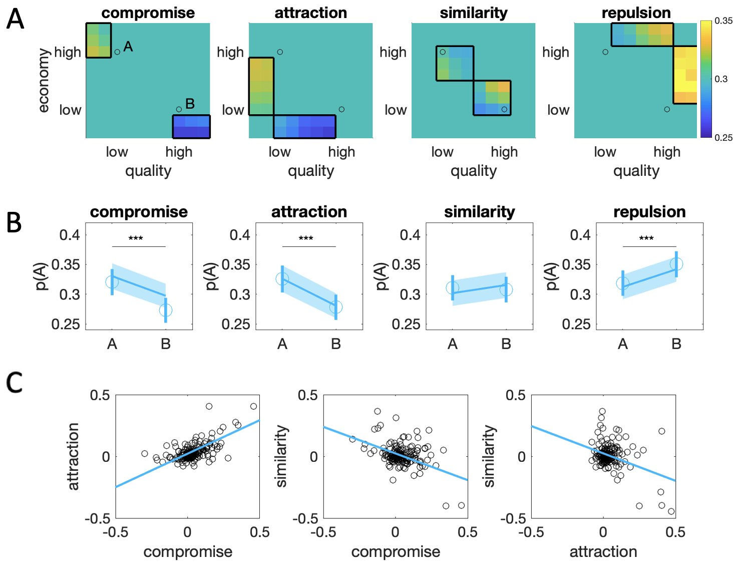
Figure 2.3: Conventional decoy analyses. \(\textbf{A:}\) Each panel illustrates the chosen locations in decoy space for compromise (\(D_c\)), attraction (\(D_a\)), similarity (\(D_s\)) and repulsion (\(D_r\)) decoys (boxes). The blue-yellow color scale illustrates relative preference for target A over B (warmer colors) or vice versa (colder colors) at each location. Black circles indicate the locations of targets A and B. \(\textbf{B:}\) Average choice share for target A as a function of decoy location across \(D_c\), \(D_a\), \(D_s\) and \(D_r\). Blue dots are human data, shaded lines are model fit of adaptive gain model (see below). Bars/shaded area signal M±SEM *** indicates p < 0.001. \(\textbf{C:}\) Correlations between the attraction, compromise and similarity effects. Each dot is a single participant; the decoy estimate is calculated as the difference between the RCS for given decoy with respect to targets A and B.
Fig. 2.3b illustrates the difference in choice share driven by decoys in the 4 locations associated with \(D_c\), \(D_a\), \(D_s\) and \(D_r\) (defined in Fig. 2.3a). As a first general observation, despite the careful sampling of targets that were matched in price/quality ratio according to participants’ responses in the valuation phase, and despite the incentives offered for consistent responding, participants exhibited a bias towards the high item B (average RCS ~ 0.7) over the low item A. Despite this additive bias, however, decoys had a clear and robust influence on choice. Participants exhibited clear attraction (\(t_{188}=4.74\), \(p<0.001\)) and compromise (\(t_{188}=6.31, p<0.001\)) effects, which were statistically significant and in the expected direction. There was also empirical support for a repulsion effect (\(t_{188}=3.45\), \(p<0.001\)) from superior decoys. On average, the presence of attraction, compromise or repulsion decoys shifted preferences from A to B by about 3-5%. However, we failed to replicate the similarity decoy effect (\(t_{188}=0.41\), \(p = 0.68\)).
2.2.2.1.1 Interrelationship of Effects
We observed a positive association between the attraction and compromise effects (\(r=0.72\), \(p<0.001\)) and a negative relation between the similarity effect and both compromise (\(r=-0.59\), \(p<0.001\)) and attraction (\(r=-0.46\), \(p<0.001\)) effects. Note that the latter correlations were observed despite the fact that in our data, the similarity effect was on average non-significant. These are shown in Fig. 2.3c.
2.2.2.1.2 Map of Decoy Influence
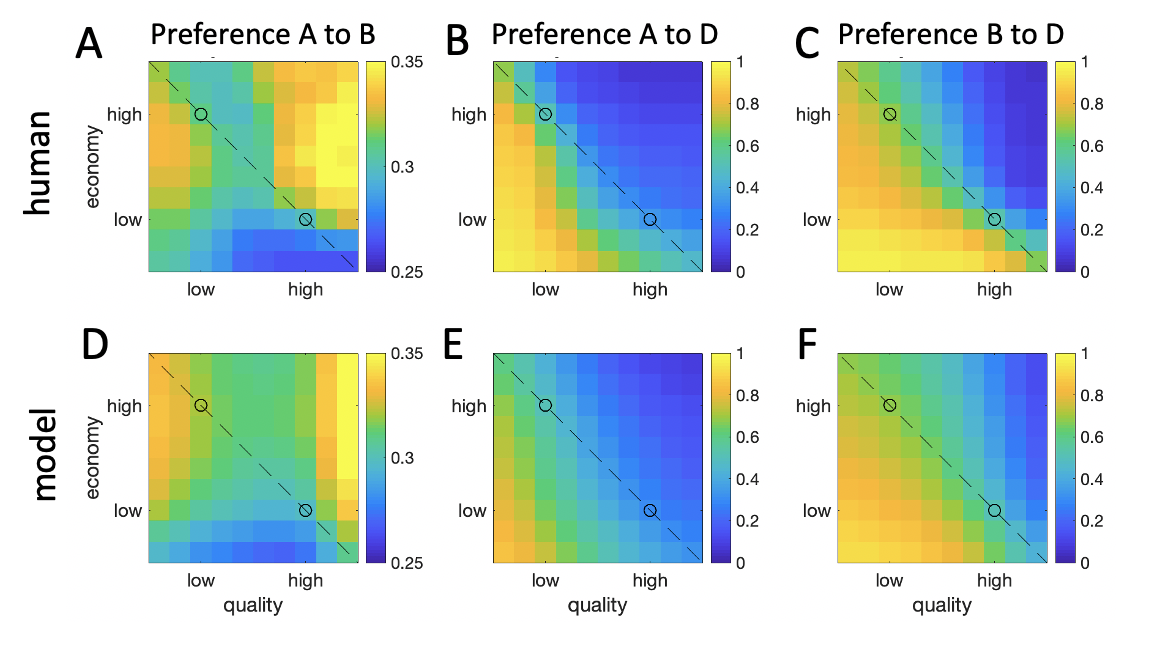
Figure 2.4: Map of decoy influence. \(\textbf{A:}\) Decoy influence map showing \(RCS_{ij}\) for A over B (left panels), A over D (middle panels) and B over D (right panels). Upper plots are the human data and lower plots are the same data for the simulated adaptive gain model (see below). The dashed line signals isopreference and the black circles are the targets A and B.
The full map of decoy influence \(RCS_{ij}\) is shown in Fig. 2.4a. Visual inspection reveals that the map has rich structure beyond the traditional decoy locations. Relative preferences for A and B seem to be driven by a dynamic of attraction and repulsion that depends on the position of the decoy with respect to each target stimulus. Robust attraction effects (whereby the presence of a decoy that is dominated by A shifts preferences towards A) were mirrored by strong repulsion effects (whereby a decoy that dominates A shifts preferences towards B). Attraction and repulsion were observed for both targets in approximate symmetry.
The map charting preference for A > D (Fig. 2.4b) is in line with the expected pattern, whereby inferior decoys, i.e. those under the left diagonal, or line of theoretical isopreference, are chosen less often (warmer colors) than superior decoys (colder colors). Similarly, the map charting preference for B > D (Fig. 2.4c) adheres to this general pattern. In theory, if A and B were equally preferred, these two maps would be identical. However, in line with the observed preference bias for the high value item B, we see that overall, preferences for A > D appear weaker compared to preferences for B > D.
2.2.2.1.3 Map Decomposition
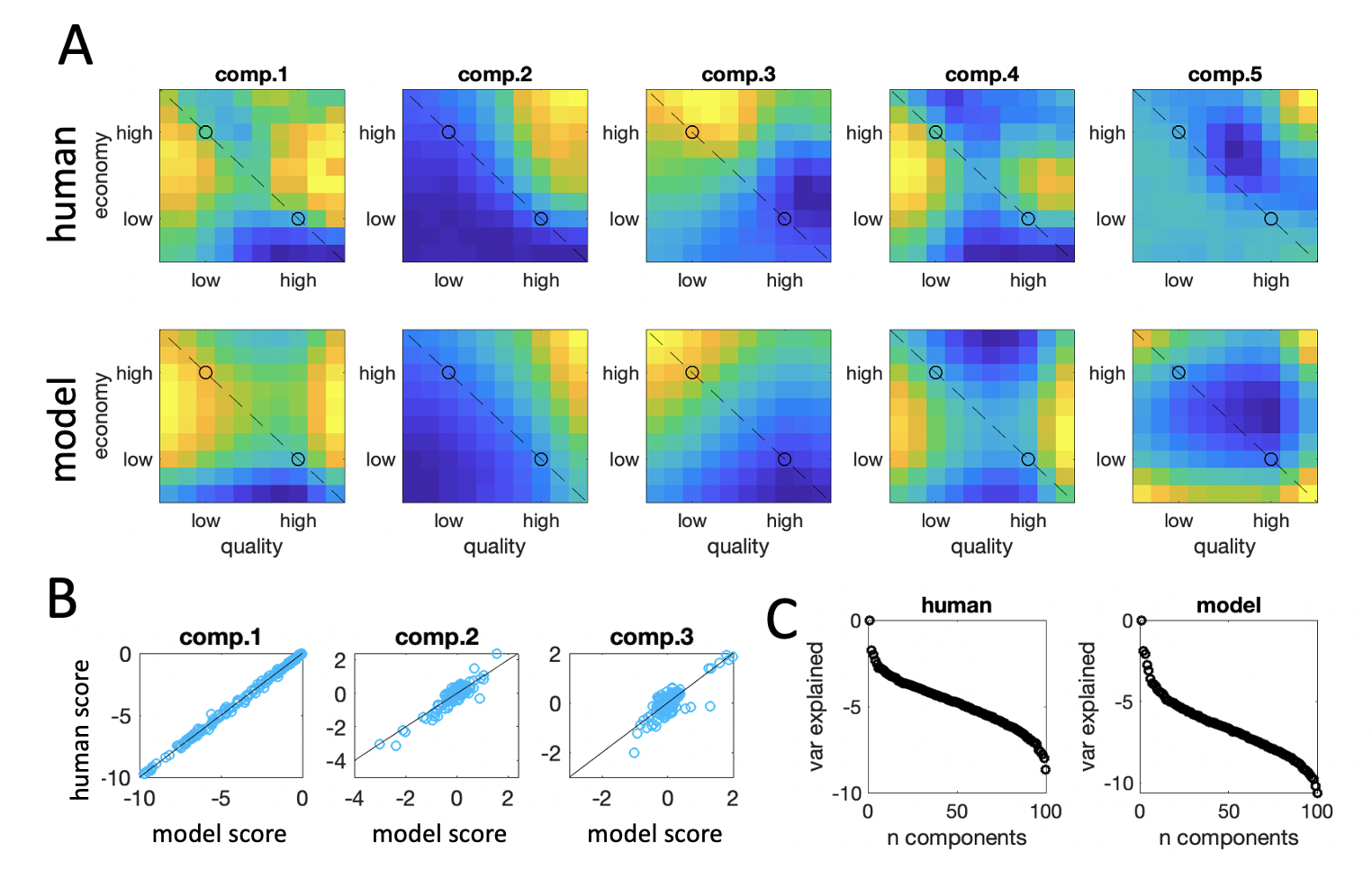
Figure 2.5: Map decomposition. \(\textbf{A:}\) First five components obtained from singular value decomposition (SVD) of the RCS for A vs. B. Upper plots are the human data and lower plots are the model. \(\textbf{B:}\) Correlation between component scores for components 1-3 between the human and the best-fitting model. For components 1-3, this correlation was very high. \(\textbf{C:}\) The variance explained by each component obtained by SVD for the humans (left panel) and the model (right panel). Note that the y-axis is on a log scale; the data is dominated by the first component in both cases.
Next, we sought to examine the structure of the map of decoy influence (Fig. 2.4a) via dimensionality reduction. The first 5 factors identified by SVD are visualized in Fig. 2.5a (top row). The first factor accounted for 95% of the variance in the data, suggesting that there is a single explanatory variable that drives decoy effects across participants (Fig. 2.5c, right panel, note the logarithmic scale on the y-axis). This finding is consistent with the correlation results reported above, showing the robust interrelationships between the three classic effects in our participants.
2.2.3 Interim Discussion
Conventional decoy analyses of our data replicated the previously extensively documented compromise and attraction effects (J. Huber, Payne, and Puto 1982; Simonson 1989). However, we failed to replicate the similarity decoy effect in this dataset, consistent with weak or absent similarity effect from other studies (Noguchi and Stewart 2014; Berkowitsch, Scheibehenne, and Rieskamp 2014). Indeed, while the attraction effect tends to be highly robust and consistent across participants, the compromise effect and similarity effects tend to be more idiosyncratic, with a high proportion of participants showing effects which are inverted with respect to the canonical form. For example, in previous studies only a minority of participants show all three effects (numerically) in the expected direction (e.g. only 23% in Trueblood, Brown, and Heathcote 2015, we find a comparable figure of 22%).
Despite the fact that the similarity effect was on average non-significant in our dataset, its strength inversely correlated with the strength of the compromise and attraction effects. Those two effects were in turn positively associated with one another. This pattern of interrelationships of the decoy effects mirrors previous reports (Noguchi and Stewart 2014) and is further supported by our results on the structure of the full map of decoy influence. In particular, we found that a single explanatory factor is sufficient to capture 95% of the variability of decoy influence in our dataset.
One interpretation of this data is that the attraction, compromise and similarity effects are not distinct phenomena, but rather they are all driven by a single common computational principle. This principle ensures that decision values of stimuli A and B are repulsed away from proximal decoys on a line which lies perpendicular to the line of isopreference, giving rise firstly to what is traditionally known as the “attraction” effect (a potentially confusing nomenclature, given that decision values for a target are repulsed away from those of the decoy) and secondly to its converse identified here for superior decoys, which we have dubbed the “repulsion” effect. The compromise and similarity effects can arise because these repulsive effects may vary in strength for targets A and B, and/or for inferior and superior decoys, such that repulsive effects “spill over” asymmetrically towards the extremes of the isopreference line (compromise effect) or into the center of the bivariate decoy map (similarity effect). It is the fact that compromise and similarity effects are really driven by asymmetric attraction and repulsion that gives rise to the strong correlations in effects across the cohort observed in this paper and previously (Berkowitsch, Scheibehenne, and Rieskamp 2014).
2.3 Computational Modeling
These findings suggest that it should be possible to identify a simple model that can reproduce the full decoy influence map with parameters that control the putative repulsive principle, as well as additional degrees of freedom that allow for asymmetric scaling of the attribute values (quality and economy). Previous simulation work demonstrated that a gain-control process can provide a unifying explanation for similar choice biases (V. Li et al. 2018). In this theoretic account, the gain with which alternatives are encoded is adaptively adjusted according to the context provided by other available options. Recent proposals of models for decoy phenomena have also appealed to a similar adaptive framework, whereby decision signals are normalized by context (Rigoli et al. 2017; Daviet 2018).
2.3.1 Adaptive Gain Model
The normalization principle in the adaptive gain model assumes that for each attribute (e.g. quality or economy), a relative value estimate is computed that reflects the distance between each item and the mean of the available choice set. We thus begin by defining \(r(A)\), which is the value of target A relative to other items, including the decoy, on a given attribute \(i\): \[\begin{equation} r(A_i) = v(A_i) - v(avg_i^{ABD}) \tag{2.1} \end{equation}\] where \(v(avg_i^{ABD})\) corresponds to the average value of the three alternatives on attribute \(i\): \[\begin{equation} v(avg_i^{ABD})=\frac{v(A_i)+v(B_i)+v(D_i)}{3} \end{equation}\] The model proposes that the subjective utility \(u(A_i)\) of target A on attribute \(i\) is computed through a logistic transformation of the relative value, as follows: \[\begin{equation} u_i(A_i) = \frac{1}{1+e^{-(r(A_i)-c_i)\cdot s^{-1}}} \tag{2.2} \end{equation}\] Thus, for each attribute, the utility of each target is given by a logistic function with slope \(s\) whose inflection point is the mean value of all items plus an additive bias term \(c\). The additive bias \(c\) can potentially vary across attributes.
The utility of target A is a weighed sum of its attributes \(i\) and \(j\), and the final decision is made by passing the utilities of all three rival stimuli through a softmax function to make a ternary choice: \[\begin{equation} u(A) = w \cdot u_i(A_i) + (1-w) \cdot u_j(A_j) \tag{2.3} \end{equation}\] \[\begin{equation} p(A) = \frac{e^{\tau u(A)}}{e^{\tau u(A)}+e^{\tau u(B)}+e^{\tau u(D)}} \tag{2.4} \end{equation}\] In addition to the softmax temperature \(\tau\), the model potentially has 4 free parameters of interest: the slope \(s\), and inflection points \(c_i\) and \(c_j\) of the logistic function Eq. (2.3), and the weighing parameter \(w\) in Eq. (2.4).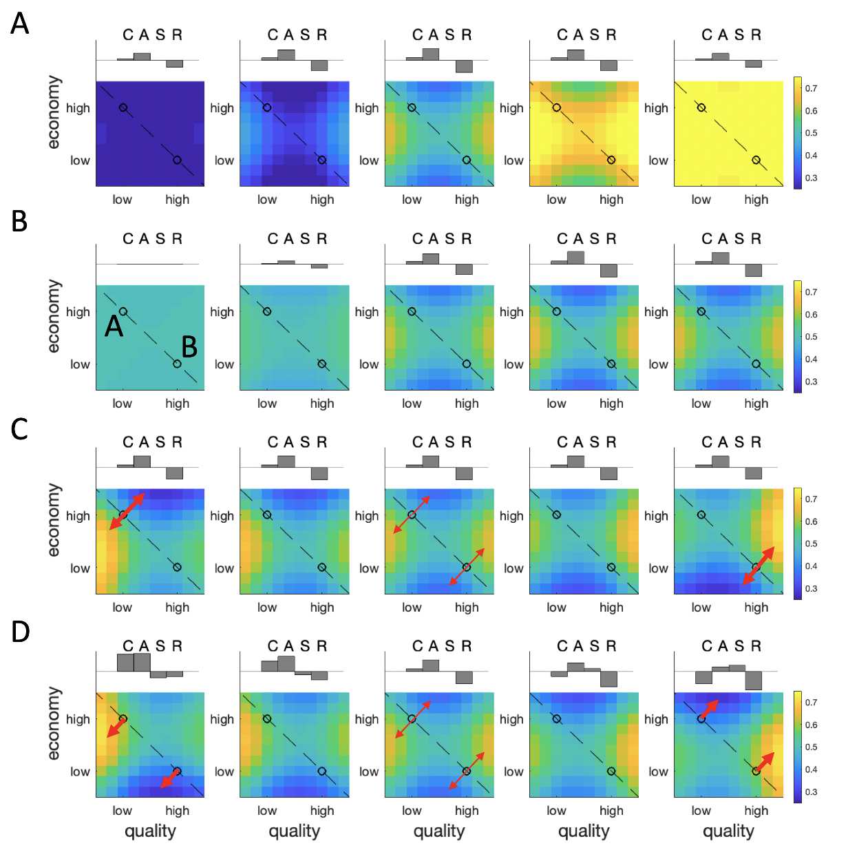
Figure 2.6: Simulated maps of decoy influence. \(\textbf{A:}\) Effect of varying the parameter \(w\) from low (left panels) to high (right panels). This parameter controls the relative preference for low price/quality to high price/quality items. \(\textbf{B:}\) The effect of varying the parameter \(s\) from high to low. This parameter controls whether A and B are equally preferred, or whether there is decoy-like distortion. \(\textbf{C:}\) The effect of varying the difference of bias terms \(c_i\)=\(-c_j\) from negative (left panels) to positive (right panels). Varying this difference alters whether the maximal distortion occurs proximal to target A (left) or target B (right). \(\textbf{D:}\) The effect of varying the sum of bias terms \(c_i=c_j\) from negative (left panels) to positive (right panels). Varying this difference alters whether the maximal distortion occurs for inferior decoys (left) or superior decoys (right). Red arrows highlight directions of repulsion, with arrow width schematically representing the strength of the effect.
2.3.1.1 Model Simulations
We explore the effects of manipulating these parameters on the predicted decoy influence map in Fig. 2.6; a full description of the parameters used is available in Table ??. This figure shows how the model can systematically account for not only the pattern observed in the current experiment, but also those from previous (and potentially contradictory) reports. In Fig. 2.6a we show the effect of manipulating the parameter \(w\). This simply shows how we can tip the balance of preferring A over B according to the relative weight given to each attribute.
In Fig. 2.6b, with \(w\) now fixed to 0.5 (equal weighing of the two attributes), we show how the decoy effects grow in strength with \(s\). Above each plot the relative positive or negative strength of the compromise (\(D_c\)), attraction (\(D_a\)), similarity (\(D_s\)) and repulsion (\(D_r\)) effects are shown in a bar plot. As can be seen, the attraction and repulsion effects grow as \(s\) grows, including a weak compromise effect but no similarity effect.
Fig. 2.6c shows the influence of varying \(c_i=-(c_j)\) while \(s\) and \(w\) are fixed. This has the effect of shifting the relative strength of the attraction/repulsion effect for targets A and B. For example, when \(c_i>c_j\) the attraction/repulsion effects are strongest for the target A, whereas when \(c_j>c_i\) they are strongest for B (red arrows). However, because these effects cancel out symmetrically, this does not affect the overall RCS for \(D_c\), \(D_a\), \(D_s\) or \(D_r\).
Finally, varying \(c_i=c_j\) (Fig. 2.6d) brings about an asymmetric distortion whereby either attraction effects are stronger (i.e. below the isopreference line) or repulsion effects are stronger (in the superior decoy portion of space). In addition to varying the relative strength of attraction and repulsion, this allows the compromise effect to vary from positive to negative, as described in previous studies; it allows a weak similarity effect to emerge. Combinations of all of these factors give the model systematic flexibility to account for a wide range of observed effects.Interestingly, the simulations shown in Fig. 2.6d allow us to make a new prediction about the human data. As seen in the bar plots accompanying each predicted influence map, when \(c_i\) and \(c_j\) are both negative, the compromise effect is positive and attraction is stronger than repulsion. By contrast, when \(c_i\) and \(c_j\) are both positive, the compromise effect is negative and the repulsion effect is stronger than attraction. The model thus predicts that on average, in the human data there will be a correlation between the (signed) compromise effect and the relative magnitude of attraction vs repulsion. This is plotted in Fig. 2.7, and as can be seen this prediction holds for the data we collected (\(r=0.57\), \(p<0.001\)). Of note, this effect was driven both by a positive correlation between the compromise effect and the strength of repulsion (\(r=0.43\), \(p<0.001\)), as well as the correlation between compromise and attraction effects described above.
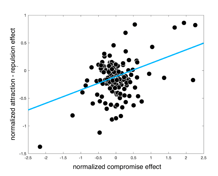
Figure 2.7: Correlation between the compromise effect and the relative strength of attraction vs repulsion in the human data. Each dot is a participant; the blue line is the best fitting linear trend.
2.3.1.2 Model Fitting
Next, we estimated the model parameters which best fit the data for each participant in our experiment to assess whether the model was able to capture the results at the individual as well as aggregate level.
2.3.1.2.1 Model Fitting Methods
The model provided predictions about probabilities of choosing option A over B, which allowed us to compute model likelihoods on each trial. Those likelihoods were then used for model fitting and comparison. We estimated the model for each participant individually using gradient descent with the globalsearch function from the MATLAB Optimization Toolbox.
2.3.1.2.2 Model Fitting Results
Fitting this 5-parameter (\(\tau\), \(s\), \(c_i\), \(c_j\), \(w\)) model to human data, we can fully recreate the decoy effects observed in this study using both conventional (Fig. 2.3b) and novel (Fig. 2.4d-f) analysis methods. Specifically, the model captured almost exactly the pattern of traditional decoy effects, in terms of the relative impact on RCS of \(D_a\), \(D_c\) and \(D_s\), as well as the repulsion decoy \(D_r\) (blue shaded lines in Fig. 2.3b). The model reproduced the pattern of preferences for target A > target B qualitatively and quantitatively across the decoy space, and when we applied SVD to the model data generated under the best-fitting parametrization for each participant, the first five components that emerged were nearly identical to those for humans, and the first model component explaining 97% of the variance (Fig. 2.5c). When we plotted the estimated singular values for the first three components for humans and the best-fitting model, we found them to be very tightly correlated (Fig. 2.5b). The model also displayed the same pattern of positive association between attraction and compromise effect (\(r=0.86\)) and negative association between the similarity and attraction (\(r=-0.85\)) and similarity and compromise effects (\(r=-0.94\)). In other words, the model captures the human data very closely, both at the individual and the aggregate level.
2.3.2 Model Comparisons
The adaptive gain model belongs to a class of models which describe contextual biases as arising from normalization among populations of neurons. Normalization models share commitment to the idea that information is divisively normalized by the local context. The precise mathematical formulation of this procedure, however, differs between theoretical accounts. Some models, for instance, use measures of the central tendency of the features present in the local context (e.g. the average of attribute values, Louie, Khaw, and Glimcher 2013), while other appeal to measures of the dispersion of features (e.g. the range of attribute values, Soltani, De Martino, and Camerer 2012). Similarly, models might encode features linearly (e.g. Bushong, Rabin, and Schwartzstein 2021) or compress them prior to normalization (e.g. via a logistic operation as in the model described here and in Rigoli 2019). Below we highlight several prominent normalization models in the literature. Our aim was to compare our model to a broad space of alternative accounts that similarly assume the value of each target (on each attribute) is encoded relative to its competitors. Thus, we began our model comparison exercise with contrasts with those well established competitors.
The classic formulation of the divisive normalization theoretical tradition (henceforth vanilla divisive normalization, VDN) can be broadly encapsulated in the following expression (Carandini and Heeger 2012; Louie, Khaw, and Glimcher 2013): \[\begin{equation} u_i(A_i)^{VDN} = \frac{v(A_i)}{v(avg_i^{ABD})+c_i} \tag{2.5} \end{equation}\] where \(c_i\) is a small regularization constant. The model assumes that decision inputs are divided by the current contextual expectation, that is, the average of all current options.
In one variant of this model, which has been recently and successfully used to account for decoy effects, this normalization is also “recurrent,” i.e. it overweighs the focal item’s contribution to normalization (Daviet 2018; Webb, Glimcher, and Louie 2021): \[\begin{equation} u_i(A_i)^{RDN} = \frac{v(A_i)}{v(A_i)+v(avg_i^{ABD})+c_i} \tag{2.6} \end{equation}\]
Note that the adaptive gain model (Eq. (2.2)) is equivalent to a form of the recurrent divisive normalization model in which the values are exponentiated prior to normalization: \[\begin{equation} u_i(A_i)^{AG} = \frac{\exp(\frac{v(A_i)}{s})}{\exp(\frac{v(A_i)}{s})+\exp(\frac{v(avg_i^{ABD})+c_i}{s})} \tag{2.6} \end{equation}\]
Alongside these two models, we also considered a class of contextual normalization, which uses the range (rather than the average) of attribute values being encoded on a given trial to normalize an imperative stimulus: \[\begin{equation} u_i(A_i)^{RN} = \beta \frac{v(A_i)}{v(rng_i^{ABD})} \tag{2.7} \end{equation}\] where \(v(rng_i^{ABD})\) corresponds to the corresponds to the difference between highest and lowest values of attribute \(i\) across all stimuli (target or decoy) in the trial and \(\beta\) is a scaling term (Soltani, De Martino, and Camerer 2012; Bushong, Rabin, and Schwartzstein 2021).
2.3.2.1 Methods
We compared the fit of each of the candidate normalization accounts to adaptive gain in a direct model comparison exercise. To achieve this, we used Bayesian model selection on cross-validated model evidence. Cross-validation involved estimating model parameters from one half of trials (by comparing fits to preferences between target items A and B, as well as preferences between target and decoys) and computing log-likelihoods from the held-out trials. We implemented this using the globalsearch function from the MATLAB Optimization Toolbox. For Bayesian model selection, we used the Statistical Parametric Mapping Toolbox (Stephan et al. 2009).
2.3.2.2 Results
Comparisons between cross-validated model likelihoods revealed that the exceedance probability for the adaptive gain model over each of the three competitor models (vanilla divisive normalization, recurrent divisive normalization and range normalization) was 0.99, providing decisive evidence for the former over each of the latter.
2.3.3 Charting Normalization Models of Decoy Influence
2.3.3.1 Grandmother Model
To go beyond those established models and compare our model to a broader range of competitors, we also devised and fit a more flexible model which encompassed a large space of possible normalization schemes. This “grandmother” model could capture the encoding scheme proposed by the 4 models introduced above, along with a number of other “hybrid” models. Thus, exploring the parameter space of the grandmother model allows us to explore the space of putative normalization schemes, including those that are yet to be described in the literature, and chart how different model features translate to predicted patterns of decoy influence.
The model had the general form:
\[\begin{equation} u_i(A_i) = \frac{1}{\beta_1 + e^{-(v(A_i)^k - \mu_i^k)(s \cdot k)^{-1}}} \tag{2.8} \end{equation}\] where \[\begin{equation} \mu_i = c_i+ \beta_2 \cdot v(avg^{ABD}_i)+(1-\beta_2)\cdot v(rng^{ABD}_i) \end{equation}\]
We focus on free parameters \(\beta_1\), \(\beta_2\), and \(k\), which respectively encode the tendency to engage in asymmetric weighing of the evaluated (recurrent) item (\(\beta_1\)), the tendency to normalize with respect to the mean vs range (\(\beta_2\)) and the extent to which inputs are compressed before being transduced (\(k\)).
Parameter \(k\) facilitated comparison between the adaptive gain model (which incorporates a logistic transformation) and other normalization models (which do not), by leveraging the following limit:
\[\begin{equation} \lim_{k \to 0} \frac{x^k-1}{k} = \log_e x, \forall x>0 \tag{2.9} \end{equation}\]
Thus, substituting \(x\) above for our variables of interest, \(v(A_i)\) and \(\mu\), we obtain:
\[\begin{equation} \log v(A_i) - \log \mu_i = \lim_{k \to 0} \frac{v(A_i)^k-1}{k}-\frac{\mu_i^k-1}{k} = \lim_{k \to 0} \frac{v(A_i)^k - \mu_i^k}{k} \tag{2.10} \end{equation}\]
Thus, \(k\) thus corresponds to the extent to which inputs are compressed before being transduced, with \(k\sim 0\) signifying a logarithmic compression, and \(k=1\) signifying linear input. Simulations revealed that implementing a value of \(k\) as high as 0.001 satisfactorily approximates the natural logarithm (Fig. 2.8).
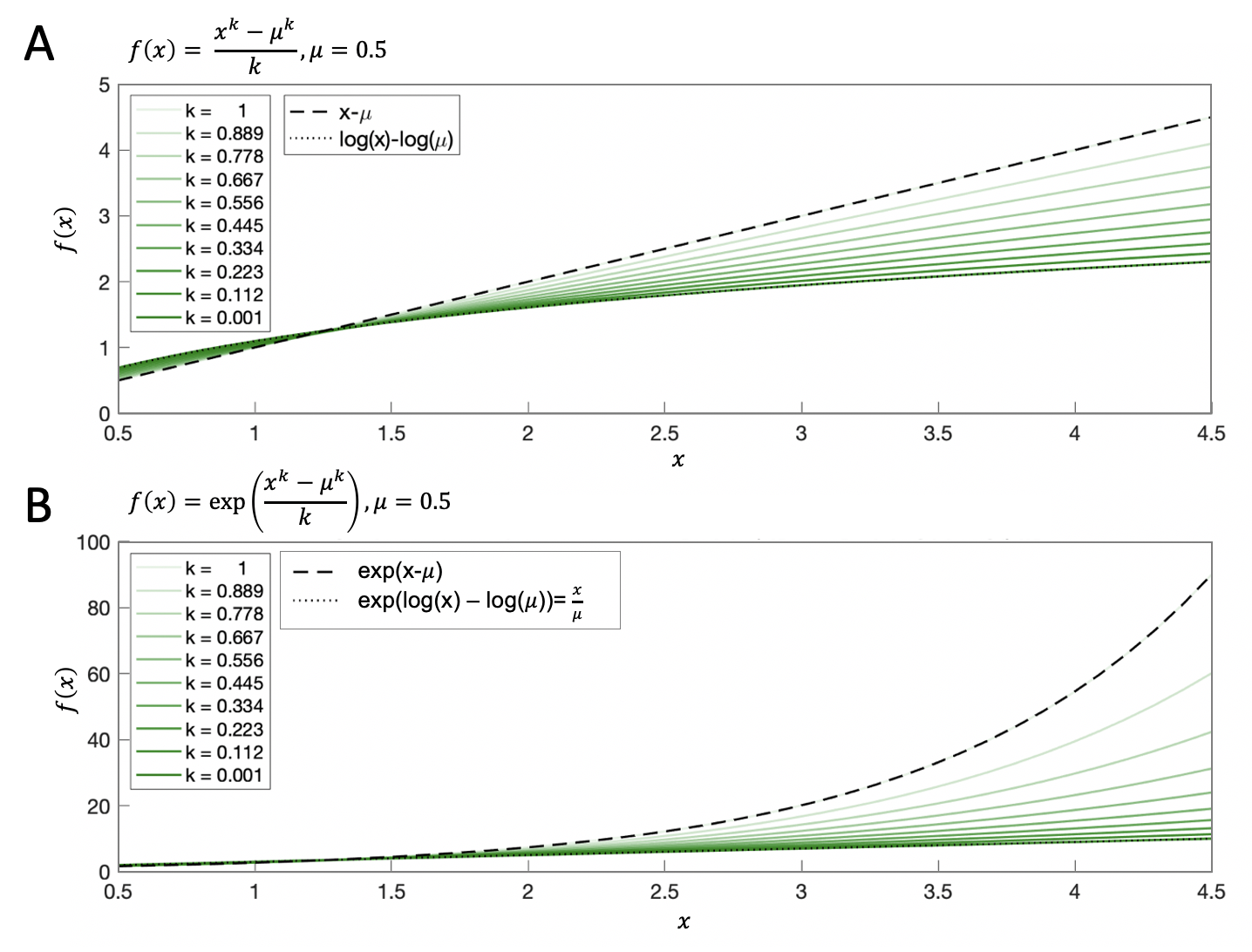
Figure 2.8: Illustration of variations in parameter \(k\). \(\textbf{A:}\) Using parameter \(k\) to interpolate between a linear expression and its logarithmic compression. Note that the darkest green curve (\(k=0.001\)) lies on the dotted line (logarithmic expression), suggesting that implementing a value of \(k\) as high as 0.001 satisfactorily approximates the natural logarithm. \(\textbf{B:}\) Exponentiating the function from panel A, as in the logistic formulation of the grandmother model. Note that the darkest green curve (\(k=0.001\)) lies on the dotted line (linear expression, \(\exp(\log(x)-\log(\mu))=\frac{x}{\mu}\)). This demonstrates that we can recover both normalization models that rely on logistic compression and normalization models that do not.
2.3.3.2 Grandmother Model Derivations
The adaptive gain, vanilla and recurrent divisive normalization, and range normalization models were nested within the grandmother model. This section shows how each of them can be derived from the general grandmother model equation.
Leveraging the limit from Eq. (2.9), when we plug in the parameter values for vanilla divisive normalization specified in Table ?? into the general grandmother model, we arrive at the formulation of vanilla divisive normalization (as per Eq. (2.5)):
\[\begin{equation} u_i(A_i) = \frac{1}{e^{-(v(A_i)^{0.001}-\mu_i^{0.001})(0.001)^{-1}}} = \frac{1}{e^{-(\log{v(A_i)}-\log{\mu_i})}} = \frac{1}{\frac{\mu_i}{v(A_i)}} = {\frac{v(A_i)}{\mu_i}} = {\frac{v(A_i)}{v(avg^{ABD}_i)+c_i}} \end{equation}\]
Similarly, we may simplify the grandmother model into recurrent divisive normalization (Eq. (2.6)) by plugging in the relevant parameter values specified in Table ??:
\[\begin{equation} \begin{aligned} u_i(A_i) = \frac{1}{1+e^{-(v(A_i)^{0.001}-\mu_i^{0.001})(0.001)^{-1}}} = \frac{1}{1+e^{-(\log{v(A_i)}-\log{\mu_i})}} = \\ \frac{1}{1+\frac{\mu_i}{v(A_i)}} = {\frac{v(A_i)}{v(A_i)+\mu_i}} = {\frac{v(A_i)}{v(A_i)+v(avg^{ABD}_i)+c_i}} \end{aligned} \end{equation}\]
Note that if we allow parameter \(s\) to vary freely, it assumes the role of a power transform for inputs:
\[\begin{equation} \begin{aligned} u_i(A_i) = \frac{1}{1+e^{-(v(A_i)^{0.001}-\mu_i^{0.001})(s \cdot 0.001)^{-1}}} = \frac{1}{1+e^{-(\log{v(A_i)}-\log{\mu_i})^{s^{-1}}}} = \\ \frac{1}{1+\frac{\mu_i^{s^{-1}}}{v(A_i)^{s^{-1}}}} = {\frac{v(A_i)^{s^{-1}}}{v(A_i)^{s^{-1}}+\mu_i^{s^{-1}}}} = {\frac{v(A_i)^{s^{-1}}}{v(A_i)^{s^{-1}}+(v(avg^{ABD}_i)+c_i)^{s^{-1}}}} \tag{2.11} \end{aligned} \end{equation}\]
Similarly, we may obtain the formulation of range normalization (Eq. (2.7)) by plugging in the relevant parameter values from Table ?? into the general grandmother model:
\[\begin{equation} u_i(A_i) = \frac{1}{e^{-(v(A_i)^{0.001}-\mu^{0.001}_i)(0.001)^{-1}}} = \frac{1}{e^{-(\log{v(A_i)}-\log{\mu_i})}} = \frac{1}{\frac{\mu_i}{v(A_i)}} = {\frac{v(A_i)}{\mu_i}} = {\frac{v(A_i)}{v(rng^{ABD}_i)}} \end{equation}\]
Finally, we may reduce the grandmother model to adaptive gain (Eq. (2.2)) by plugging in the relevant parameter values from Table ??:
\[\begin{equation} \begin{aligned} u_i(A_i) = \frac{1}{1+e^{-(v(A_i)-\mu_i) \cdot s^{-1}}} = \frac{1}{1+e^{-({v(A_i)}-{\mu_i}) \cdot s^{-1}}} = \frac{1}{1+e^{-({v(A_i)}-v(avg^{ABD}_i)-c_i)\cdot s^{-1}}} \end{aligned} \end{equation}\]
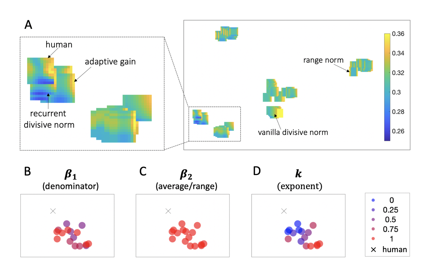
Figure 2.9: Charting decoy models. \(\textbf{A:}\) Embedding space for normalization models of decoy effects. A \(t\)-distributed stochastic neighbour visualization of the maps of decoy influence produced by different variants of the grandmother model. Each map represents a variant of the grandmother model positioned in 2D space such that models with similar decoy influence patterns are nearby, while models with more different decoy patterns are further apart. Heat maps illustrate decoy influence. The rectangle on the left shows a zoomed in version of the denoted subset of embedding space. \(\textbf{B-D:}\) These plots depict the zoomed in subset of embedding space presented above. Each model-produced decoy map is denoted as a dot and color coded to indicate parameter value: \(\beta_1\) (panel B), \(\beta_2\) (panel C), or \(k\) (panel D). Human data is represented with a cross.
Note that along with those specific models, which have been described in the literature, there exist many more parametrizations of the grandmother model which correspond to “hybrid” normalization schemes, combining specific features of the above described accounts.
2.3.3.3 Fitting the Grandmother Model
2.3.3.3.1 Methods
We fit 125 variations of the grandmother model, by varying \(\beta_1\) and \(\beta_2\) in 5 steps between 0 and 1, and \(k\) in 5 steps between 0.001 and 1, in addition to the four constrained parametrizations of the grandmother model that result in the vanilla divisive normalization, recurrent divisive normalization, adaptive gain and range normalization models (Table ??). We used the \(t\)-distributed stochastic neighbor embedding (t-SNE) visualization technique (Van Der Maaten and Hinton 2008) to calculate relations among the resulting decoy influence maps from the 129 parametrizations. We specified the t-SNE hyperparameter perplexity, which controls the number of expected close neighbors, following guidelines in the literature to balance the trade-off between perplexity and the Kullback–Leibler divergence (Cao and Wang 2017).
2.3.3.3.2 Results
Fitting the grandmother model to human data revealed the different patterns of decoy influence predicted by variations of the general coding scheme. The embedding plot in Fig. 2.9a shows the simulated decoy maps for each of the 129 parametrizations of the grandmother model. Neighboring maps reflect models that produce relatively similar patterns of decoy influence (and vice versa for distant points). In Fig. 2.9b-d the points are colored according to levels of \(\beta_1\), \(\beta_1\) and \(k\), revealing the human data is neighbored by maps generated by models with high values of parameters \(\beta_1\) and \(\beta_2\), i.e. those that resemble the adaptive gain model.
We note that the precise value of parameter \(k\), which interpolates between models implementing logistic and linear divisive normalization, is less important for fitting human data. This implies that the model is equally well fit with an exponentiated implementation of recurrent divisive normalization (\(k = 1\), such as the adaptive gain model) and with a linear implementation of recurrent divisive normalization (\(k\) ~ \(0\)), where inputs are transformed with a power parameter \(s\) prior to normalization (\(s\neq 0\), see Eq. (2.11)). This latter formulation of recurrent divisive normalization (as in Eq. (2.11)) is conceptually analogous to a form of recurrent divisive normalization in which values are power transformed (as in Daviet 2018): \[\begin{equation} u_i(A_i)^{PRDN} = \frac{v(A_i)^{\alpha}}{v(A_i)^{\alpha}+v(avg_i^{ABD})^{\alpha}+c_i} \tag{2.12} \end{equation}\]
Indeed, Bayesian model selection reveals that this model fits the data equally well as the adaptive gain model (exceedance probability for PRDN = 0.49), suggesting that our dataset cannot arbitrate between an exponential and power transform of attribute values.
Why is the nonlinear compression of attribute values important? To explore the role of this procedure, we compared the maps of decoy influence produced by an implementation of the grandmother model incorporating a logistic (i.e. exponential) transform of attribute values (equivalent to the adaptive gain model) and an implementation of the grandmother model incorporating attribute values linearly (equivalent to recurrent divisive normalization without a power transform) in Fig. 2.10a. The nonlinearity qualitatively changes the form of the decoy map. The model featuring linearly coded attribute values produces stronger contextual effects for decoys of higher attribute values. This result can be traced back to the shape of the transducer function under linear attribute values (Fig. 2.10b, red curve), which is a non-symmetric concave function. Consequently, the curve deviates more from the identity line along the higher end of the abscissa and this leads to higher distortions in the translation of higher compared lower attribute values.
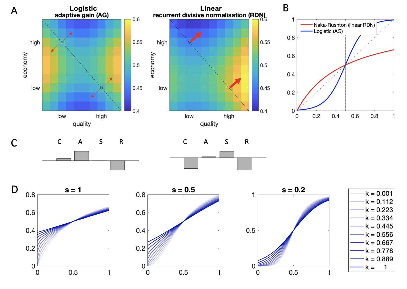
Figure 2.10: The role of the compressive nonlinearity. \(\textbf{A:}\) Simulated decoy maps for the adaptive gain and recurrent divisive normalization models. It is noteworthy that the adaptive gain model (with bias terms \(c_i=c_j=0\)) produces symmetric regions of repulsion and attraction around the line of isopreference. By contrast, “linear” recurrent divisive normalization (i.e. RDN without a power transform applied to values prior to transduction) produces stronger repulsion and attraction for superior decoys (i.e. decoys above rather than below the isopreference line). \(\textbf{B:}\) The asymmetric pattern of decoy influence seen for linear RDN occurs because the transducer is a (decelerating) Naka-Rushton function. This function is concave, meaning that the derivative is always higher (i.e. curve steeper) for low than high attribute values irrespective of the value of \(x\). By contrast, the transducer for AG is sigmoidal and it is thus symmetric around the midpoint (which is itself adjusted to the context; this is the “adaptive” part). This panel plots the transductions applied to inputs by the Naka-Rushton function in red and by the Sigmoidal function in blue, with \(v((avg)_i)=0.5\) (dashed line), \(s=0.1\). The recurrent divisive normalization framework (without additional nonlinearity) implies that those attribute values which are always relatively smaller (closer to zero) are processed with higher gain. By contrast, the adaptive gain model implies that resources are allocated preferentially to the mean of a context, exaggerating binary distinctions which potentially straddle that midpoint (e.g. “low” vs. “high” value). \(\textbf{C:}\) The relative strengths of the compromise, attraction, similarity and repulsion effects per the two decoy maps. \(\textbf{D:}\) Illustration of the transfer function of the grandmother model, with \(c_i=c_j=0\), \(\beta_1=\beta_2=1\), and \(v((avg)_i)=0.5\), across different values of \(k\) and \(s\). Note that with this parametrization, the transducer function is equivalent to a logistic function when \(k=1\), and to a Naka-Rushton function when \(k \sim 0\) and \(s=1\). Power transforming inputs (by setting \(s \neq 1\)) in the Naka-Rushton definition approximates the sigmoidal shape of the adaptive gain transducer.
This is in contrast to what happens in the presence of an exponential nonlinearity as in the adaptive gain model. This compression of attribute values produces an S-shaped transducer (Fig. 2.10b, blue curve), akin to the sigmoidal shapes of response functions ubiquitous in neural coding. Notably, this transducer is symmetric around the inflection point (which corresponds to the mean of attribute values of the context when \(c_i=0\)) and thus results in equal levels of distortion across the low and high end of attribute space. The bias term \(c_i\) can tip the balance in either direction: it can produce stronger effects for higher attribute values when \(c_i>0\) and stronger effects for lower attribute values when \(c_i<0\) (see Fig. 2.6d for simulations). Of note, the sigmoidal shape of the transducer here can be approximated by power transforming inputs prior to normalizing them in the recurrent divisive normalization scheme (i.e. \(s>0\) and \(k\sim 0\), Fig. 2.10d lightest blue curve). This result helps clarify why this operation can capture the human data equally well as the exponential nonlinearity in the adaptive gain model.
Finally, we asked whether the adaptive gain model fits better than the full grandmother model after appropriate penalization for complexity. A failure to do so would imply the existence of a “hybrid” normalization solution that fits the human data even better, presumably involving some combination of parameters that has yet to be described in the literature. To asses this, we performed Bayesian model selection on complexity-penalized model fit metrics (Bayesian Information Criterion, BIC) which revealed that the exceedance probability for the normalization scheme favored by our empirical data, the adaptive gain model, over the grandmother model is 0.97, offering evidence against a hybrid solution.
2.3.4 Interim Discussion
Altogether, the results of our modeling suggest that a very simple computational scheme appealing to the relative encoding of attribute values may capture the full pattern of decoy influence in our dataset. We identified a 5-parameter model, previously termed adaptive gain, which fit the data exceptionally well, both at a fine scale (at the level of effects in individual participants) and on the aggregate level (the average map of decoy influence). We compared this model to related theoretical accounts in the literature, which appeal to a contextual normalization of attribute values, first, via conventional model selection techniques and second, through a comprehensive model comparison exercise for which we devised a flexible “grandmother” model encompassing a wide space of putative normalization schemes. The results of our computational work indicated that the rich pattern of decoy influence is best accounted for by information processing schemes that compressively transduce inputs, appealing to normalization by the central tendency of context and recurrently overweighing the contribution of the target input to the normalization.
2.4 Discussion
Decoy effects have been studied for decades, but substantial controversy has surrounded their replicability, interrelationship, and computational origins. This chapter sheds new light on these debates by gathering and analyzing a large-scale dataset that systematically maps the influence of a decoy stimulus across both the inferior and superior locations of multiattribute space. Conducting our analysis in a conventional fashion, we broadly replicate past studies, in that we find strong attraction effects, strong compromise effects, and a weaker and more variable similarity effect (not significant in our dataset). As in previous studies, the three decoy effects are correlated across the cohort, with a positive relationship observed between attraction and compromise, and a negative relationship between those two and the strength of the similarity effect (Berkowitsch, Scheibehenne, and Rieskamp 2014). This finding implies that three decoy phenomena have a single cause, and indeed previous dynamic models (in which information is accumulated over time) have been able to capture the three discrete effects with a single set of parameters (Roe, Busemeyer, and Townsend 2001; Usher and McClelland 2004; Bhatia 2013; Trueblood, Brown, and Heathcote 2014; Bhui and Gershman 2018). Here, we use dimensionality reduction on the full decoy influence map to confirm that indeed, there is a single component that explains the vast majority (~95%) of the variance in decoy influence, suggestive of a single computational origin for these biases.
To understand the computational origin of decoy effects, we chose to model our data with a framework based on divisive normalization. We made this choice because the normalization model offers a simple, parsimonious account of contextual biases in decision-making based on a rich, neurobiologically grounded tradition in the cognitive sciences (Carandini and Heeger 2012; Louie, Khaw, and Glimcher 2013; Rigoli 2019; Landry and Webb 2021; Webb, Glimcher, and Louie 2021). In particular, it allowed us to systematically measure the influence of various candidate computational steps on the predicted decoy map, providing an interpretable mapping from model to data (Fig. 2.6). On this basis, we were able to establish (for example) that normalization occurs relative to the average of the available values (via a sigmoidal gain function) rather than to the lower end (via a concave gain function) as proposed in some previous models (Fig. 2.10). This characteristic sigmoidal shape of the transfer function may be approximated by transforming inputs via a power term (\(\alpha>1\)) in recurrent divisive normalization (Daviet 2018; Webb, Glimcher, and Louie 2021).
Overall, out of the models tested here, evidence favored a model that has previously been described in the literature as the adaptive gain model (Cheadle et al. 2014; V. Li et al. 2018). This account is closely related to other models involving recurrent divisive normalization, especially those proposing that values are nonlinearly transformed beforehand, as well as being very similar to another model known as the logistic model of subjective value (Rigoli 2019). There is a close correspondence between qualitative features of model-simulated and human performance displayed in Fig. 2.4, and in particular, a close correspondence achieved after decomposition of the decoy map into linear components using singular value decomposition (Fig. 2.5). The adaptive gain model even predicted a new and potentially counter-intuitive relationship between the decoy effects: that when the compromise effect is positive, attraction should dominate over repulsion (and vice versa), a prediction that was satisfied in the data.
Under the adaptive gain control framework described here, decoy effects occur because of contextual biases arising when each target item is transduced via a logistic function whose inflection point lies at the mean of all three items including the decoy. For example, the “attraction” effect thus occurs because when the decoy is lower in value than item A, the inflection point is lower than item A, and so A lies at the steepest portion of the sigmoidal gain function and is thus “overvalued” or repulsed away from this mean point. The precise converse occurs when the decoy is higher in value than A, as well as for B. Previous work has demonstrated that exactly this mechanism can in principle account for a range of decision biases arising in the presence of distractors, across perceptual, cognitive and economic domains (V. Li et al. 2018). The brain may have evolved the type of normalization scheme proposed here because it promotes efficient neural coding (Summerfield and Tsetsos 2015, 2020).
Whereas the attraction effect tends to be highly robust and consistent across participants, the strength and directionality of the compromise effect and similarity effects tend to be more idiosyncratic. Indeed, the similarity effect did not reach statistical significance in our dataset. In our model, the compromise and similarity effects occur when attractive and repulsive processes are asymmetric due to differential weighing or biasing of the two attributes, causing attraction effects (and their converse for superior decoys) to warp and/or “spill over” into locations where compromise and similarity decoys are typically tested. In other words, the fragile nature of the compromise and similarity effects might be at least in part due to heterogeneity in the asymmetric way each attribute is coded or transformed, which in turn might (for example) be due to differing choice concerning stimulus materials. A systematic unpicking of ways in which different classes of stimulus material (e.g. numerical values in distinct ranges, perceptual stimuli such as rectangles, and vignettes) are encoded, and thus why decoy effects may or may not have emerged in previous studies (Frederick, Lee, and Baskin 2014; Joel Huber, Payne, and Puto 2014; Spektor, Bhatia, and Gluth 2021), is beyond the scope of our research project here. However, our simulations suggest that a relatively low-dimensional encoding model may be sufficient to capture this variation and thus to pinpoint the source of variation in previous studies.
2.5 Conclusion
Adding a “decoy” alternative to a choice set can shift preferences in multialternative economic decisions. A long research tradition focusing on this contextual bias has provided evidence for three classic decoy effects – the compromise, attraction and similarity effects – but their replicability, interrelationship and computational origins have sparked controversy. To address these, we carried out a large-scale incentive-compatible study, charting the full two dimensional attribute space of decoy effects. Our analyses indicated that a single explanatory factor can account for the rich pattern of decoy influence we observe. Indeed, a simple process model, appealing to the principle of divisive normalization, can capture our results both at the individual and aggregate level.
2.6 Acknowledgements
This chapter is based on the published work Dumbalska, T., Li, V., Tsetsos, K., & Summerfield, C. (2020). A map of decoy influence in human multialternative choice. Proceedings of the National Academy of Sciences, 117(40), 25169-25178.
The human data for this chapter was procured by Dr Vickie Li. Dr Vickie Li and Prof Christopher Summerfield jointly designed and Dr Vickie Li built the experiment and administered data collection. Dr Konstantinos Tsetsos provided feedback on code for the modeling simulations.